FIBAD Demonstration

For this demonstration we’ll walk through a simplified version of a typical machine learning workflow supported by FIBAD.

import fibad  # The primary package for this demo

import pooch  # Used to retrieve example data
import chromadb  # Used to explore the vector database

import numpy as np
import matplotlib.pyplot as plt

import subprocess
from pathlib import Path
from IPython.display import IFrame

# Helper functions for data retrieval and plotting
from fibad.config_utils import find_most_recent_results_dir
from mpr_demo_plotting import sort_objects_by_median_distance, plot_grid

Download a sample HSC dataset

file_path = pooch.retrieve(
    # DOI for Example HSC dataset
    url="doi:10.5281/zenodo.14498536/hsc_demo_data.zip",
    known_hash="md5:1be05a6b49505054de441a7262a09671",
    fname="example_hsc_new.zip",
    path="./data",
    processor=pooch.Unzip(extract_dir="."),
)

This dataset is comprised of approximately 993 cutouts from the Hyper Suprime Cam survey. Each cutout includes i, r and g bands and is 8 arcseconds on a side.

Create and configure a FIBAD object

f = fibad.Fibad()

[2025-02-10 14:54:18,010 fibad:INFO] Runtime Config read from: /Users/drew/code/fibad/src/fibad/fibad_default_config.toml

An instance of the Fibad class will be used through out this demo. Under the hood when it is created, it will:

• Load the configuration file specified (here it’s using the built-in default).

• Parse the configuration file for external libraries and add those to the appropriate registries.

• Prepare logging for the system.

# Specify the location of the data to use for training
f.config["general"]["data_dir"] = "./data/hsc_8asec_1000"

# Specify the dataset class that represents the data
f.config["data_set"]["name"] = "HSCDataSet"
f.config["data_set"]["train_size"] = 0.8
f.config["data_set"]["validate_size"] = 0.2
f.config["data_set"]["test_size"] = 0.0

# Select the model to use for training
f.config["model"]["name"] = "ExampleAutoencoder"

# Set the number of epochs and batch size for training.
f.config["train"]["epochs"] = 20
f.config["data_loader"]["batch_size"] = 32

The default configuration needs a few tweaks to work for this demo. We’ve updated the location of our sample data, and specified which model we want to train.

The configuration is represented as nested python dictionary. This allows for easy manipulation in a notebook via the .config attribute of the fibad instance.

Train a model

f.train()

[2025-02-10 16:30:01,634 fibad.data_sets.hsc_data_set:INFO] Processed 993 objects for pruning
[2025-02-10 16:30:01,634 fibad.data_sets.hsc_data_set:INFO] Checking file dimensions to determine standard cutout size...
[2025-02-10 16:30:01,642 fibad.data_sets.hsc_data_set:INFO] HSC Data set loader has 993 objects
[2025-02-10 16:30:01,649 fibad.data_sets.hsc_data_set:INFO] test split contains 0 items
[2025-02-10 16:30:01,654 fibad.data_sets.hsc_data_set:INFO] train split contains 794 items
[2025-02-10 16:30:01,656 fibad.data_sets.hsc_data_set:INFO] validate split contains 199 items
[2025-02-10 16:30:01,668 fibad.models.model_registry:INFO] Using criterion: torch.nn.MSELoss with arguments: {'reduction': 'none'}.
2025-02-10 16:30:01,669 ignite.distributed.auto.auto_dataloader INFO: Use data loader kwargs for dataset '<fibad.data_sets.hsc':
        {'sampler': <torch.utils.data.sampler.SubsetRandomSampler object at 0x17cf2bc90>, 'batch_size': 32, 'num_workers': 2, 'pin_memory': False}
2025-02-10 16:30:01,670 ignite.distributed.auto.auto_dataloader INFO: Use data loader kwargs for dataset '<fibad.data_sets.hsc':
        {'sampler': <torch.utils.data.sampler.SubsetRandomSampler object at 0x350f62310>, 'batch_size': 32, 'num_workers': 2, 'pin_memory': False}
2025/02/10 16:30:01 WARNING mlflow.system_metrics.system_metrics_monitor: Skip logging GPU metrics because creating `GPUMonitor` failed with error: Failed to initialize NVML, skip logging GPU metrics: NVML Shared Library Not Found.
2025/02/10 16:30:01 INFO mlflow.system_metrics.system_metrics_monitor: Started monitoring system metrics.
[2025-02-10 16:30:01,707 fibad.pytorch_ignite:INFO] Training model on device: mps

[2025-02-11 10:01:53,340 fibad.pytorch_ignite:INFO] Total training time: 63111.63[s]
[2025-02-11 10:01:53,343 fibad.pytorch_ignite:INFO] Latest checkpoint saved as: /Users/drew/code/mpr_fibad/results/20250210-163001-train-tQru/checkpoint_epoch_20.pt
[2025-02-11 10:01:53,344 fibad.pytorch_ignite:INFO] Best metric checkpoint saved as: /Users/drew/code/mpr_fibad/results/20250210-163001-train-tQru/checkpoint_18_loss=-168.1707.pt
2025/02/11 10:02:03 INFO mlflow.system_metrics.system_metrics_monitor: Stopping system metrics monitoring...
2025/02/11 10:02:03 INFO mlflow.system_metrics.system_metrics_monitor: Successfully terminated system metrics monitoring!
[2025-02-11 10:02:03,401 fibad.train:INFO] Finished Training

When we call .train() to train the model there’s a lot going on under the hood:

• The model is automatically loaded onto the fastest hardware available.

• A data loader is instantiated and configured to load batches of data to the same hardware.

• A new timestamped directory is created under the configured results directory where all output is saved.

• The configuration becomes immutable and a copy is saved for reproducibility.

• The model and system metrics start being logged for review in both TensorBoard and MLFlow.

• Checkpoints are saved automatically both at the last epoch and at the epoch with the lowest loss value.

• Finally, the model weights file is saved.

Training time depends heavily on the hardware available, model, and training parameters. For a point of reference, training takes about 40s for this case:

• Model trained: Built-in autoencoder

• Dataset and size: Example HSC data, 993 samples, 96x96 pixel cutouts

• Number of epochs: 20

• Batch size: 32

• Hardware: Desktop with GTX 1660 Super GPU

While we train on only about 1,000 samples here, FIBAD training has scaled up to over 1M samples on an HPC system with access to multiple GPUs without requiring the user to make any code changes. To do so, the command line interface of FIBAD was used to work within a Slurm environment like so:

>> fibad train --runtime-config ./results/<timestamped_directory>/runtime_config.toml

Quickly evaluate the model

%reload_ext tensorboard
%tensorboard --logdir {f.config['general']['results_dir']}

The preceding cell will start TensorBoard, to perform simple evaluation of trained models. While TensorBoard can run easily in a notebook, when that notebook is rendered to HTML (for demonstration or documentation) the server backing the TensorBoard UI isn’t included in the rendering. If the cell above was run locally, the resulting UI would look similar to the following screen shot.

Create a new model

import torch.nn as nn
from fibad.models.model_registry import fibad_model


@fibad_model  # This decorator registers the model with the FIBAD framework
class TrialAutoencoder(nn.Module):
    def __init__(self, config, shape):
        super().__init__()
        self.config = config

        # Encoder
        self.encoder = nn.Sequential(
            nn.Conv2d(3, 16, kernel_size=3, stride=2, padding=1),  # (16, 48, 48)
            nn.ReLU(),
            nn.Conv2d(16, 32, kernel_size=3, stride=2, padding=1),  # (32, 24, 24)
            nn.ReLU(),
            nn.Conv2d(32, 64, kernel_size=3, stride=2, padding=1),  # (64, 12, 12)
            nn.ReLU(),
            nn.Conv2d(64, 128, kernel_size=3, stride=2, padding=1),  # (128, 6, 6)
            nn.ReLU(),
        )

        # Decoder
        self.decoder = nn.Sequential(
            nn.ConvTranspose2d(128, 64, kernel_size=3, stride=2, padding=1, output_padding=1),  # (64, 12, 12)
            nn.ReLU(),
            nn.ConvTranspose2d(64, 32, kernel_size=3, stride=2, padding=1, output_padding=1),  # (32, 24, 24)
            nn.ReLU(),
            nn.ConvTranspose2d(32, 16, kernel_size=3, stride=2, padding=1, output_padding=1),  # (16, 48, 48)
            nn.ReLU(),
            nn.ConvTranspose2d(16, 3, kernel_size=3, stride=2, padding=1, output_padding=1),  # (3, 96, 96)
            nn.Sigmoid(),  # Normalize output to [0, 1]
        )

    def _eval_encoder(self, x):
        return self.encoder(x)

    def _eval_decoder(self, x):
        return self.decoder(x)

    def forward(self, x):
        return self._eval_encoder(x)

    def train_step(self, x):
        z = self._eval_encoder(x)
        x_hat = self._eval_decoder(z)

        loss = self.criterion(x, x_hat)
        loss = loss.sum(dim=[1, 2, 3]).mean(dim=[0])
        self.optimizer.zero_grad()
        loss.backward()
        self.optimizer.step()
        return {"loss": loss.item()}

New models can be written in a notebook for easier experimentation. Above, an autoencoder is written for comparison against the built-in ExampleAutoencoder where the only difference is that the built-in autoencoder uses nn.GeLU while nn.ReLU is used here.

Note that the class is decorated with @fibad_model, this decorator automatically provides several conveniences for the user:

• The model class is registered with FIBAD for training.

• Default loss and optimizer functions are provided.

• Support for defining loss and optimizer functions in the FIBAD configuration.

• Methods to save and load model weights are provided included.

• Automatic verification that required methods were implemented.

In addition to the @fibad_model, other decorators to support extensibility and reduce boilerplate code have been developed, including:

• @fibad_dataset - for rapid development of new data set interfaces

• @fibad_verb - for new core actions i.e. f.custom_train(...), f.bespoke_predict(...), etc.

Train the newly defined model

# Specify that we now want to train the model defined in this notebook
f.config["model"]["name"] = "TrialAutoencoder"

# Define loss and optimizer functions for easy experimentation
f.config["criterion"]["name"] = "torch.nn.MSELoss"
f.config["torch.nn.MSELoss"] = {"reduction": "none"}

f.config["optimizer"]["name"] = "torch.optim.Adam"
f.config["torch.optim.Adam"] = {"lr": 1e-3}

# train the new model
f.train()

[2025-02-10 16:12:09,170 fibad.data_sets.hsc_data_set:INFO] Processed 993 objects for pruning
[2025-02-10 16:12:09,171 fibad.data_sets.hsc_data_set:INFO] Checking file dimensions to determine standard cutout size...
[2025-02-10 16:12:09,172 fibad.data_sets.hsc_data_set:INFO] HSC Data set loader has 993 objects
[2025-02-10 16:12:09,174 fibad.data_sets.hsc_data_set:INFO] test split contains 0 items
[2025-02-10 16:12:09,175 fibad.data_sets.hsc_data_set:INFO] train split contains 794 items
[2025-02-10 16:12:09,175 fibad.data_sets.hsc_data_set:INFO] validate split contains 199 items
[2025-02-10 16:12:09,178 fibad.models.model_registry:INFO] Using criterion: torch.nn.MSELoss with arguments: {'reduction': 'none'}.
[2025-02-10 16:12:09,178 fibad.models.model_registry:INFO] Using optimizer: torch.optim.Adam with arguments: {'lr': 0.001}.
2025-02-10 16:12:09,179 ignite.distributed.auto.auto_dataloader INFO: Use data loader kwargs for dataset '<fibad.data_sets.hsc':
        {'sampler': <torch.utils.data.sampler.SubsetRandomSampler object at 0x3190431d0>, 'batch_size': 32, 'num_workers': 2, 'pin_memory': False}
2025-02-10 16:12:09,179 ignite.distributed.auto.auto_dataloader INFO: Use data loader kwargs for dataset '<fibad.data_sets.hsc':
        {'sampler': <torch.utils.data.sampler.SubsetRandomSampler object at 0x351b94a50>, 'batch_size': 32, 'num_workers': 2, 'pin_memory': False}
2025/02/10 16:12:09 WARNING mlflow.system_metrics.system_metrics_monitor: Skip logging GPU metrics because creating `GPUMonitor` failed with error: Failed to initialize NVML, skip logging GPU metrics: NVML Shared Library Not Found.
2025/02/10 16:12:09 INFO mlflow.system_metrics.system_metrics_monitor: Started monitoring system metrics.
[2025-02-10 16:12:09,230 fibad.pytorch_ignite:INFO] Training model on device: mps

[2025-02-10 16:29:28,011 fibad.pytorch_ignite:INFO] Total training time: 1038.78[s]
[2025-02-10 16:29:28,013 fibad.pytorch_ignite:INFO] Latest checkpoint saved as: /Users/drew/code/mpr_fibad/results/20250210-161209-train-q4OZ/checkpoint_epoch_20.pt
[2025-02-10 16:29:28,014 fibad.pytorch_ignite:INFO] Best metric checkpoint saved as: /Users/drew/code/mpr_fibad/results/20250210-161209-train-q4OZ/checkpoint_17_loss=-130.8977.pt
2025/02/10 16:29:38 INFO mlflow.system_metrics.system_metrics_monitor: Stopping system metrics monitoring...
2025/02/10 16:29:38 INFO mlflow.system_metrics.system_metrics_monitor: Successfully terminated system metrics monitoring!
[2025-02-10 16:29:38,049 fibad.train:INFO] Finished Training

Note the adjustments that were made to f.config before beginning the training. First the model name is updated to be the name of the new model class defined in this notebook. Recall that the @fibad_model decorator will register the model with FIBAD, this is what allows us to refer to the model by the class name.

Additionally we defined the loss and optimizer functions in the config to be used by the model. FIBAD supports this feature to allow easy experimentation and evaluation of the performance of these hyperparameters.

Compare multiple models

# Start the MLFlow UI server
backend_store_uri = f"file://{Path(f.config['general']['results_dir']).resolve() / 'mlflow'}"
mlflow_ui_process = subprocess.Popen(
    ["mlflow", "ui", "--backend-store-uri", backend_store_uri, "--port", "8080"],
    stdout=subprocess.PIPE,
    stderr=subprocess.PIPE,
)

# Display the MLFlow UI in an IFrame in the notebook
IFrame(src="http://localhost:8080", width="100%", height=1000)

FIBAD automatically logs training information for model evaluation. Here we see an in-notebook instance of the MLFlow UI. Typically, the UI would be started from the command line and viewed in a browser to avoid having to scroll back and forth in a notebook. The typical command to do so would look like: mlflow ui --backend-store-uri <results_directory/mlflow>

While MLFlow can run in a notebook, when that notebook is rendered to HTML (for demonstration or documentation) the server backing the MLFlow UI isn’t included in the rendering. If the cell above was run locally, the resulting UI would look similar to the following screen shot.

Running inference

# Update the data set splits to be 100% test data
f.config["data_set"]["test_size"] = 1.0
f.config["data_set"]["train_size"] = 0.0
f.config["data_set"]["validate_size"] = 0.0

# Increase batch size for faster inference
f.config["data_loader"]["batch_size"] = 512

# Run inference
f.infer()

[2025-02-10 15:31:20,454 fibad.data_sets.hsc_data_set:INFO] Processed 993 objects for pruning
[2025-02-10 15:31:20,455 fibad.data_sets.hsc_data_set:INFO] Checking file dimensions to determine standard cutout size...
[2025-02-10 15:31:20,457 fibad.data_sets.hsc_data_set:INFO] HSC Data set loader has 993 objects
[2025-02-10 15:31:20,458 fibad.data_sets.hsc_data_set:INFO] test split contains 993 items
[2025-02-10 15:31:20,459 fibad.data_sets.hsc_data_set:INFO] train split contains 0 items
[2025-02-10 15:31:20,462 fibad.models.model_registry:INFO] Using criterion: torch.nn.MSELoss with arguments: {'reduction': 'none'}.
[2025-02-10 15:31:20,462 fibad.models.model_registry:INFO] Using optimizer: torch.optim.Adam with arguments: {'lr': 0.001}.
[2025-02-10 15:31:20,462 fibad.infer:INFO] data set has length 993
2025-02-10 15:31:20,463 ignite.distributed.auto.auto_dataloader INFO: Use data loader kwargs for dataset '<fibad.data_sets.hsc':
        {'sampler': None, 'batch_size': 512, 'num_workers': 2, 'pin_memory': False}
[2025-02-10 15:31:20,619 fibad.pytorch_ignite:INFO] Evaluating model on device: mps
[2025-02-10 15:31:20,620 fibad.pytorch_ignite:INFO] Total epochs: 1
[2025-02-10 15:31:36,819 fibad.pytorch_ignite:INFO] Total evaluation time: 16.20[s]
[2025-02-10 15:31:46,828 fibad.infer:INFO] Inference results saved in: /Users/drew/code/mpr_fibad/results/20250210-153120-infer-pOl_

For this demo, we’ll pretend that of all the models we trained, the last one performed best. We’ll now use that model to run inference. Note that by default, FIBAD will find the weights of the last successfully trained model for inference, but of course, a different set of weights can be specified in the configuration.

Aside: What does “inference” mean?

The term “inference” simply means to pass data through a trained model to produce an output.

First we make a small update to the data set splits, setting test_size to 100% and the other splits to 0%. We also increase the batch size in order to make better use of the available GPU memory.

Finally we run inference over the dataset using the trained model weights with f.infer(). As with training, FIBAD is doing a lot behind the scenes including:

• Freezing the configuration and saving a copy for reproducibility.

• Saving the results of inference in batched .npy files.

• Optionally persisting the results to a vector database.

Again, while predicting the latent space for only 1,000 samples here, FIBAD inference has scaled up to over 1M samples on an HPC system with access to multiple GPUs without requiring any code changes.

Exploring the results of inference

# Establish a connection to the database containing the inference results
results_dir = find_most_recent_results_dir(f.config, "infer")
client = chromadb.PersistentClient(path=str(results_dir))
collection = client.get_collection("fibad")

# For each entry in the database, find the L2 norm distance to the k nearest neighbors
all_embeddings = collection.get(include=["embeddings"])
all_nn = collection.query(query_embeddings=all_embeddings["embeddings"], n_results=5)

# Calculate the median distance to the k nearest neighbor for each entry
median_dist_all_nn = np.median(all_nn["distances"], axis=1)

# Plot a histogram of the median distances
plt.figure(figsize=(12, 6))
plt.hist(median_dist_all_nn, bins=100, range=(0, 30_000))
plt.xlabel("Median distance to k nearest neighbors")
plt.ylabel("Count")
plt.show()

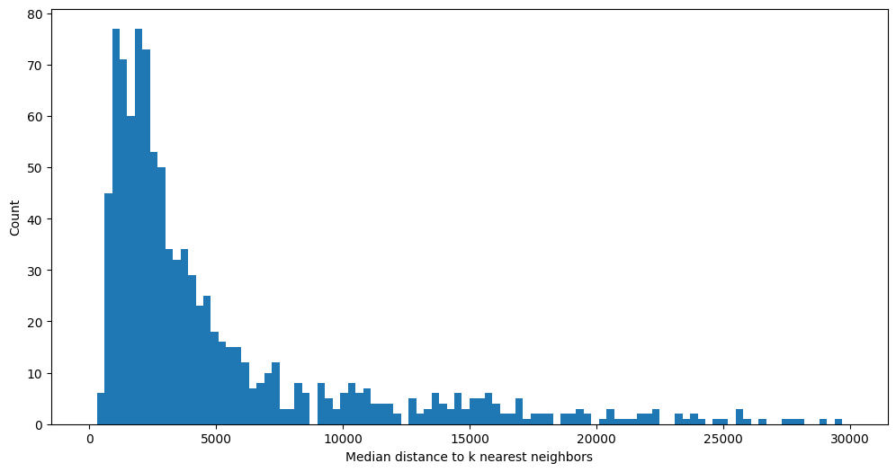
With inference complete, we can begin to explore the results. Here we make use of the built-in vector database that enables fast, approximate, similarity search. The vector database was populated automatically while running inference.

Aside: What is a “vector database”?

A vector database is one which supports efficient look ups of nearest neighbors in multidimensional space. This can be used to find the approximate K nearest neighbors for a given vector. Commercially, vector databases are often used in recommendation engines and for similarity search.

By making use of our vector database, we have:

• Efficiently found the L2 norm distance to each of the k nearest neighbors for every vector produced by inference.

• Calculated the median of the distances to the k nearest neighbors.

• Plotted the histogram of those median values.

There appears to be a long tail in the distribution of values, indicating that there are a small number of objects with latent space vectors that have median L2 norm distances much greater than the average.

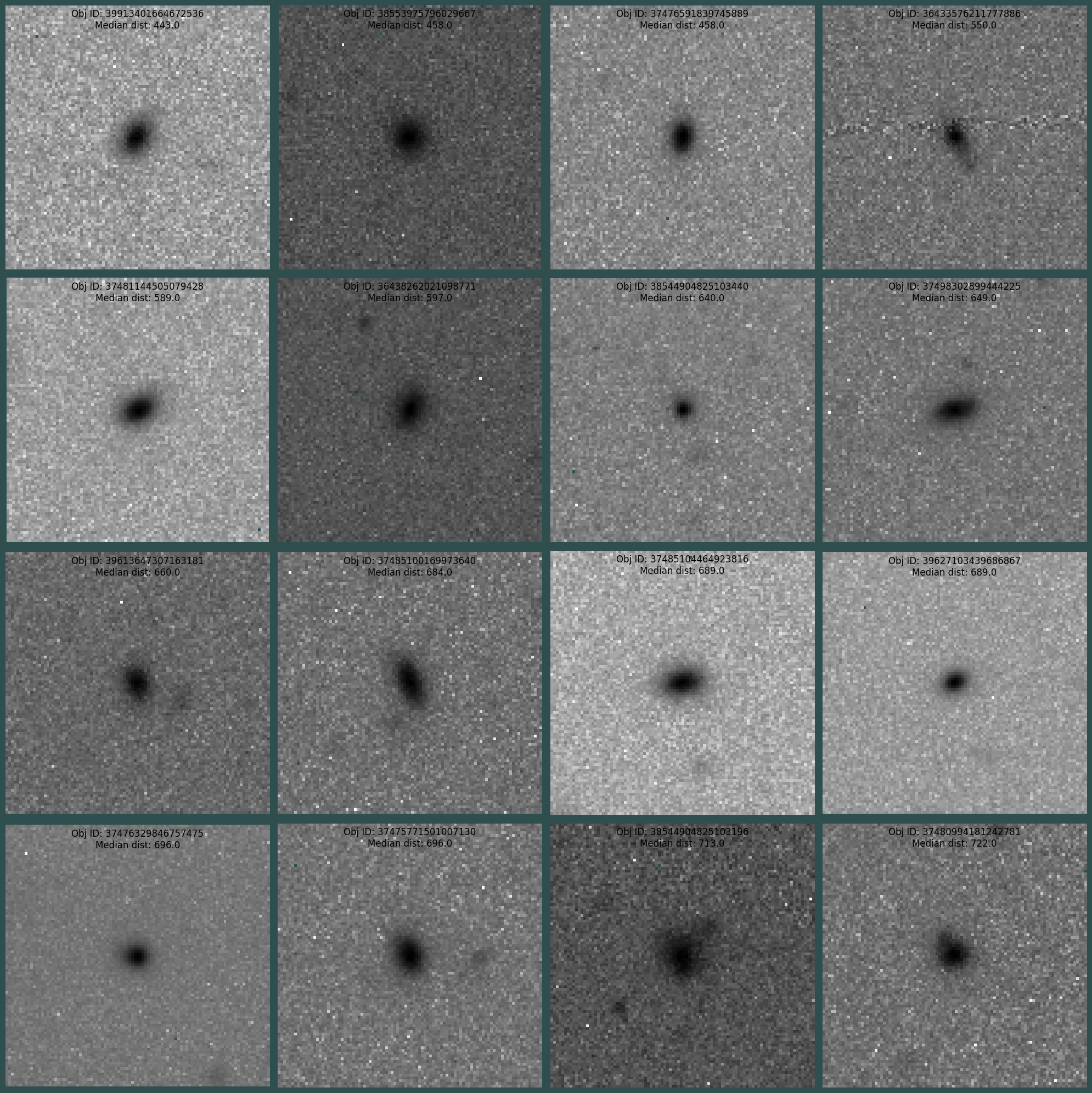
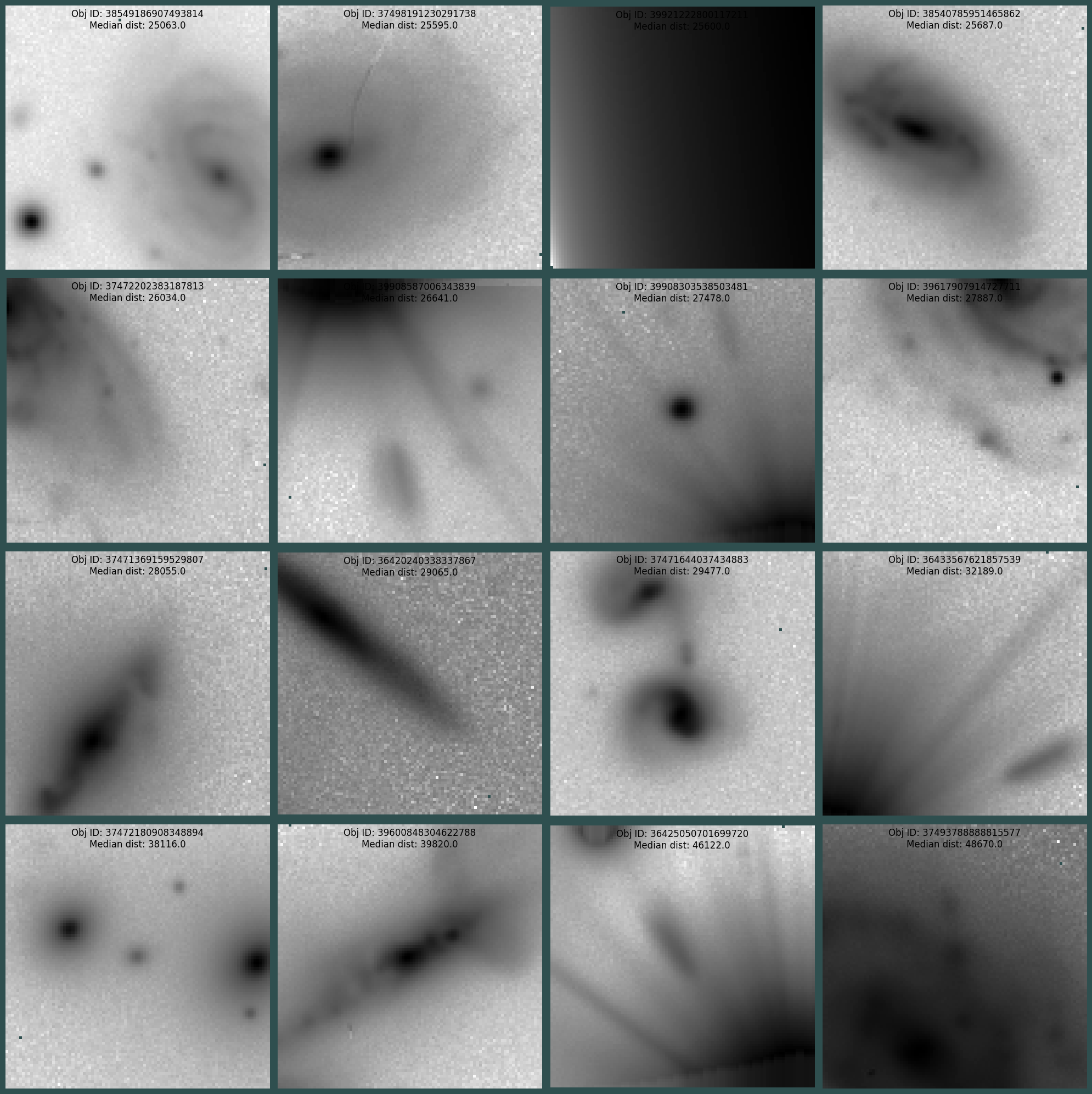
Examine a few objects

sorted_object = sort_objects_by_median_distance(
    all_embeddings, median_dist_all_nn, data_directory=f.config["general"]["data_dir"]
)

Here we order the results of the median calculation and transform the results a bit to make it easier to visualize (gather filename and median distance values for plotting). Next we plot the first and last 16 objects in the sorted list. The first 16 objects are those that correspond to near the peak of the histogram. The last 16 objects are those in the long tail of the histgram.

plot_grid(sorted_object[:16])

plot_grid(sorted_object[-16:])

Interactive visualization

f.umap()
f.visualize()

Here we are using the output of the latest inference run to inform a umap-learn fitter and produce a lower dimensional representation of the data for plotting.

The FIBAD visualization tooling utilizes Holoviews, Datashader, Bokeh and an efficient tree structure to enable the display of millions of points. It allows for panning, zooming as well as lasso and box selections. When selecting points, the resulting object ids are displayed are displayed in the associated table.

While this is an early version of interactive visualization, it has been scaled up to millions of data points. The next steps for this tooling will be to support deeper interactivity, namely:

• Automatically displaying the object selected in the table

• Leveraging the vector db to identify similar objects

• Supporting three dimensional UMAP output

This visualization runs in a notebook but when rendered to HTML (for demonstration or documentation) the server backing the interactive visual isn’t packaged with the rendering. If the cell above was run locally, the resulting UI would look similar to the following screen shot.