Author: LINCC Frameworks team

Last updated: February 10, 2025

Demo: HATS and LSDB

In this notebook we’ll show how to:

• Import DASK client

• Load object and source catalogs (lazily)

• Show HATS partitioning with ZTF objects and sources

• Perform crossmatching with existing HATS catalogs across the whole sky

• Discuss the performance

There is also an “Extra topics” section with details on margin caches.

# %pip install -q -r requirements.txt

# Standard library imports
import os
# Set to the maximum number of threads you want to allow
os.environ["NUMEXPR_MAX_THREADS"] = "128"
# Set to the number of threads to actually use
os.environ["NUMEXPR_NUM_THREADS"] = "128"

# Third-party imports
import numpy as np
import pandas as pd
import dask
from dask.distributed import Client
import matplotlib as mpl
import matplotlib.pyplot as plt
from matplotlib import rcParams
import astropy.units as u
from astropy.coordinates import SkyCoord, Angle
import warnings
import logging
from upath import UPath

# Local library-specific imports
import hats
import lsdb
from lsdb.core.search import ConeSearch
from hats.io.file_io import read_parquet_metadata
from hats.inspection import plot_density

# Jupyter-specific settings and magic commands
%matplotlib inline

# Configuration settings
warnings.simplefilter("ignore")
logging.getLogger("numexpr.utils").setLevel(logging.WARNING)
logging.getLogger("distributed").setLevel(logging.WARNING)
rcParams["savefig.dpi"] = 550
rcParams["font.size"] = 20
plt.rc("font", family="serif")
mpl.rcParams["axes.linewidth"] = 2
dask.config.set({"dataframe.convert-string": False})

print(f"Version of lsdb is {lsdb.__version__}")

Version of lsdb is 0.4.6.dev9+g7b1ec80

# Define the six fields from Data Preview 1 with RA and Dec coordinates
fields = {
    "ECDFS": (53.13, -28.10),  # Extended Chandra Deep Field South
    "EDFS": (59.10, -48.73),  # Euclid Deep Field South
    "Rubin_SV_38_7": (37.86, 6.98),  # Low Ecliptic Latitude Field
    "Rubin_SV_95_-25": (95.00, -25.00),  # Low Galactic Latitude Field
    "47_Tuc": (6.02, -72.08),  # 47 Tuc Globular Cluster
    "Fornax_dSph": (40.00, -34.45)  # Fornax Dwarf Spheroidal Galaxy
}

# Define a 2-degree (2*3600 arcseconds) search radius
radius_arcsec = 2 * 3600  # Convert 2 degree to arcseconds
# Create six cone searches
cones = {name: ConeSearch(ra=ra, dec=dec, radius_arcsec=radius_arcsec) for name, (ra, dec) in fields.items()}

Import DASK client

client = Client(n_workers=120, memory_limit="20GiB", threads_per_worker=1)

# Print the dashboard link and port
print(f"Dask is running at: {client.dashboard_link}")

Dask is running at: http://127.0.0.1:8787/status

Get GAIA and ZTF data

We have numerous public catalogs available through `data.lsdb.io <https://data.lsdb.io>`__.

catalogs_dir = UPath("https://data.lsdb.io/hats")

# Gaia
gaia_path = catalogs_dir / "gaia_dr3" / "gaia"

# ZTF
ztf_object_path = catalogs_dir / "ztf_dr14" / "ztf_object"
ztf_source_path = catalogs_dir / "ztf_dr14" / "ztf_source"
ztf_object_margin_path = catalogs_dir / "ztf_dr14" / "ztf_object_10arcs"

%%time

# Define a 0.7 degree cone region of interest
# This covers the so called `Rubin_SV_95_-25` field, one of Data Preview 1 fields
cone_search = ConeSearch(ra=95, dec=-25, radius_arcsec=0.7 * 3600)

# Load lite version of Gaia DR3 (RA and DEC data only)
gaia_lite = lsdb.read_hats(gaia_path, columns=["ra", "dec"], search_filter=cone_search)

# Load all Gaia data
hats_gaia = hats.read_hats(gaia_path)
gaia = lsdb.read_hats(gaia_path, columns=hats_gaia.schema.names)

CPU times: user 2.98 s, sys: 1.26 s, total: 4.23 s
Wall time: 4.82 s

Lazy Operations

When working with large datasets, there is too much data to be loaded into memory at once. To get around this, LSDB uses the HATS format which partitions a catalog into HEALPix cells and works on one partition at a time. This also allows the computation to be parallelized to work on multiple partitions at once. In order to efficiently carry out pipelines of operations though, it’s better to batch operations so that multiple operations can be done back to back on the same partition instead of having to load and save each partition from storage after every operation.

For this reason, operations in LSDB are performed ‘lazily’. This means when a catalog is read using read_hats, the actual catalog data isn’t being read from storage. Instead, it only loads the metadata such as the column schema and the HEALPix structure of the partitions. When an operation like cone_search is called on a catalog, the data is not actually loaded and operated on when the line of code is executed. Instead, the catalog keeps track of the operations that it needs to perform so the entire pipeline can be efficiently run later. This also allows us to optimize the pipeline by only loading the partitions that are necessary. For example when performing a cone search like we do here, we only need the partitions that have data within the cone.

So when we look at a catalog that has been lazy loaded we see the DataFrame without the data, just the columns and the number of partitions (including the HATS index of each partition encoding which HEALPix cell the partition is in).

gaia_lite

lsdb Catalog gaia:

	ra	dec
npartitions=4
Order: 3, Pixel: 321	double[pyarrow]	double[pyarrow]
Order: 3, Pixel: 323	...	...
Order: 4, Pixel: 1298	...	...
Order: 4, Pixel: 1304	...	...

The catalog has been loaded lazily, meaning no data has been read, only the catalog schema

To load the data and perform the operations, call compute() which will load the necessary data and perform all the operations that have been called, and return a Pandas DataFrame with the results.

gaia_lite_computed = gaia_lite.compute()

gaia_lite_computed

	ra	dec
_healpix_29
1450053251443354521	95.230932	-25.656355
1450053367513191047	95.277507	-25.651934
1450053378321175871	95.30161	-25.644577
1450053383016209000	95.287129	-25.646628
1450053421112786341	95.266282	-25.64857
...	...	...
1468182838101340038	95.405117	-24.405863
1468182862390320916	95.394776	-24.401534
1468182869776685320	95.387285	-24.399478
1468182870336026869	95.385895	-24.397842
1468182870426027146	95.385674	-24.397763

30372 rows × 2 columns

HATS (Hierarchal Adaptive Tiling Scheme) Partitioning

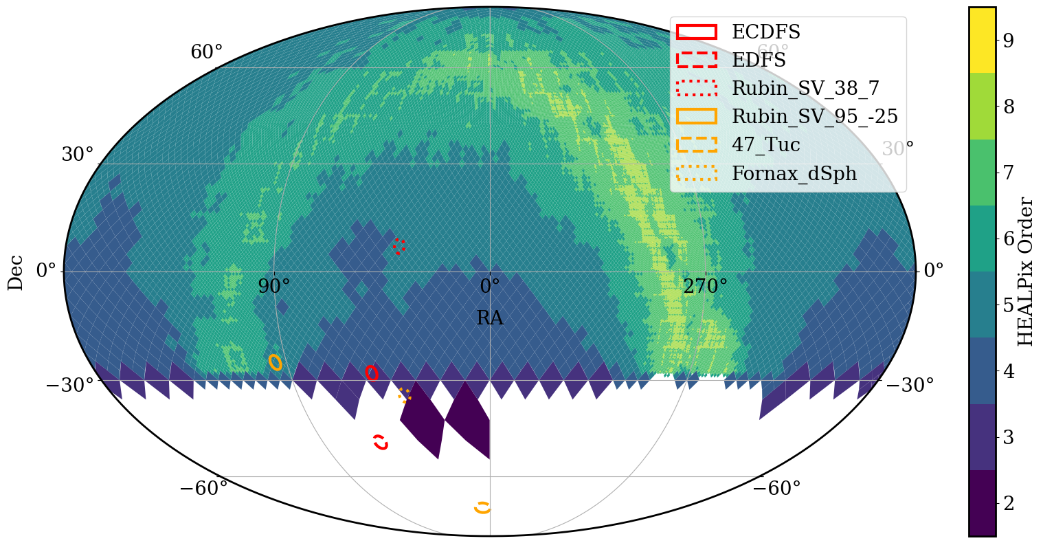
To make it easier and more efficient to perform operations in parallel, HATS partitions contain roughly the same number of rows. This is done by using different HEALPix pixel sizes for different parts of the sky depending on the density of sources. This means catalogs with more rows will have smaller pixels for each partition, and so will have more partitions overall. We can see this below with the ZTF object and source catalogs, where the source catalog with many more data points has more partitions to keep the size of each partition consistent.

%%time
ztf_object = lsdb.read_hats(ztf_object_path, columns=["ra", "dec"])  # ZTF Object
ztf_source = lsdb.read_hats(ztf_source_path, columns=["ra", "dec"])  # ZTF Source

CPU times: user 4.3 s, sys: 715 ms, total: 5.02 s
Wall time: 5.42 s

# Catalog is only lazy loaded
ztf_object

lsdb Catalog ztf_dr14:

	ra	dec
npartitions=2352
Order: 3, Pixel: 0	double[pyarrow]	double[pyarrow]
Order: 3, Pixel: 1	...	...
...	...	...
Order: 4, Pixel: 3070	...	...
Order: 4, Pixel: 3071	...	...

The catalog has been loaded lazily, meaning no data has been read, only the catalog schema

# This catalog is also only lazy loaded. Note how many more partitions it has.
ztf_source

lsdb Catalog ztf_source:

	ra	dec
npartitions=41679
Order: 4, Pixel: 0	double[pyarrow]	double[pyarrow]
Order: 4, Pixel: 1	...	...
...	...	...
Order: 5, Pixel: 12286	...	...
Order: 5, Pixel: 12287	...	...

The catalog has been loaded lazily, meaning no data has been read, only the catalog schema

We can see this difference in partition pixel sizes by plotting the HEALPix pixels of the partitions in the catalogs.

# Assign colors and linestyles
# Red for extragalactic fields, orange for dense fields
field_styles = {
    "ECDFS": ("red", "solid"),
    "EDFS": ("red", "dashed"),
    "Rubin_SV_38_7": ("red", "dotted"),
    "Rubin_SV_95_-25": ("orange", "solid"),
    "47_Tuc": ("orange", "dashed"),
    "Fornax_dSph": ("orange", "dotted"),
}

# Create the figure
fig = plt.figure(figsize=(20, 10))

# Plot the pixel density map for the ZTF object
_, ax = ztf_object.plot_pixels(fig=fig)

# Loop through all six fields and plot them with assigned colors and linestyles
for name, cone in cones.items():
    color, linestyle = field_styles[name]  # Get assigned color and linestyle
    cone.plot(edgecolor=color, facecolor="none", label=name, linewidth=3, linestyle=linestyle)

# Add a legend to distinguish the different fields (positioned in the upper right)
plt.legend(loc="upper right")

# Show the plot
plt.show()

# Plot the pixel density map for ZTF sources
# Create the figure
fig2 = plt.figure(figsize=(20, 10))

# Plot the pixel density map for the ZTF object
_, ax = ztf_source.plot_pixels(fig=fig2)

# Loop through all six fields and plot them with assigned colors and linestyles
for name, cone in cones.items():
    color, linestyle = field_styles[name]  # Get assigned color and linestyle
    cone.plot(edgecolor=color, facecolor="none", label=name, linewidth=3, linestyle=linestyle)

# Add a legend to distinguish the different fields (positioned in the upper right)
plt.legend(loc="upper right")

# Show the plot
plt.show()

Crossmatching across the whole sky

We are now ready to do a crossmatch between ZTF and GAIA. Let us try to find ZTF objects that have more than 50 detections in both r- and g- bands, and let us select FGK dwarf stars (with temperature, surface gravity, and parallax cuts). We will use power of Parquet and load only the columns that we need, which will substantially speed up the analysis.

%%time
# Load ZTF and specify the margin cache (see extra topics at the end)!
ztf_object_full = lsdb.read_hats(ztf_object_path, margin_cache=ztf_object_margin_path, columns=["ra", "dec", 'nobs_g', 'nobs_r'])

# Load Gaia DR3 with columns we need
gaia_ra_dec = lsdb.read_hats(gaia_path, columns=["ra", "dec", "parallax", 'parallax_over_error', 'teff_gspphot', 'logg_gspphot', 'classprob_dsc_combmod_star'])

CPU times: user 1.81 s, sys: 811 ms, total: 2.62 s
Wall time: 3.2 s

%%time
# Crossmatch ZTF + Gaia + filter to get FGK dwarf stars
_all_sky_object = gaia_ra_dec.crossmatch(ztf_object_full).query(
    "nobs_g_ztf_dr14 > 50 and nobs_r_ztf_dr14 > 50 and \
    parallax_gaia > 0 and parallax_over_error_gaia > 5 and \
    teff_gspphot_gaia > 5380 and teff_gspphot_gaia < 7220 and logg_gspphot_gaia > 4.5 \
    and logg_gspphot_gaia < 4.72 and classprob_dsc_combmod_star_gaia > 0.5"
)

CPU times: user 12 s, sys: 2.31 s, total: 14.3 s
Wall time: 9.69 s

%%time
gaia_ztf_xmatch = _all_sky_object.compute()

CPU times: user 2min 47s, sys: 1min 34s, total: 4min 22s
Wall time: 4min 47s

# This is the dataframe with all the computed objects
gaia_ztf_xmatch

	ra_gaia	dec_gaia	parallax_gaia	parallax_over_error_gaia	teff_gspphot_gaia	logg_gspphot_gaia	classprob_dsc_combmod_star_gaia	ra_ztf_dr14	dec_ztf_dr14	nobs_g_ztf_dr14	nobs_r_ztf_dr14	_dist_arcsec
_healpix_29
2648782300079	44.920804	0.146074	0.379842	5.828582	5441.6387	4.6079	0.999968	44.92078	0.146099	375	391	0.124185
4126993545342	44.998582	0.230765	0.734424	9.088769	5562.0205	4.6799	0.999931	44.998712	0.230687	53	53	0.545267
7287751982789	45.022036	0.286649	0.832968	23.93877	5628.6826	4.5486	0.999976	45.022041	0.286656	378	390	0.03062
9619733950647	44.781045	0.257446	0.369344	8.980508	6150.834	4.5204	0.99997	44.781049	0.257469	307	318	0.083385
21357880302975	45.374304	0.527956	1.282698	33.8478	5382.6323	4.6647	0.999956	45.374321	0.527966	379	393	0.070051
...	...	...	...	...	...	...	...	...	...	...	...	...
3458762522613795145	314.913278	-0.182307	0.489425	6.823739	5554.819	4.5722	0.999972	314.913277	-0.182287	240	309	0.072312
3458763114722019350	314.851618	-0.130918	1.148185	45.20368	6219.467	4.535	0.999913	314.851624	-0.130898	241	310	0.076127
3458763586145119598	314.966705	-0.120701	0.476298	5.975645	5498.387	4.6116	0.999988	314.966705	-0.120677	240	305	0.086584
3458763719668126460	315.055708	-0.09108	0.413605	5.472423	5383.711	4.6066	0.999973	315.055702	-0.091064	240	306	0.060258
3458763847989763944	315.032739	-0.075784	0.320514	6.255071	5604.1304	4.536	0.999987	315.032745	-0.075767	241	310	0.066412

5869703 rows × 12 columns

Ok, almost 6 million objects! Let us now visualize the GAIA object that got matched in a small patch of the sky. Orange circle shows the cone contaning one of the galactic Rubin Data Preview 1 fields.

# Extract the center coordinates from the cones dictionary for Rubin_SV_95_-25
ra_center, dec_center = cones["Rubin_SV_95_-25"].ra, cones["Rubin_SV_95_-25"].dec
center = SkyCoord(ra=ra_center * u.deg, dec=dec_center * u.deg, frame="icrs")

# Create the figure
plt.figure(figsize=(10, 8))

# Main scatter plots
plt.scatter(gaia_ztf_xmatch["ra_gaia"].values, gaia_ztf_xmatch["dec_gaia"].values, color="black", s=2, label="ZTF-GAIA Crossmatched")

# Plot a 1-degree radius circle around the center
circle_coord = center.directional_offset_by(
    position_angle=np.linspace(0, 360, 100) * u.deg, separation=0.7 * u.deg
)
plt.plot(circle_coord.ra.deg, circle_coord.dec.deg, color="orange", lw=3, label="Rubin SV_95_-25 field")

# Ensure axis limits are set correctly (adjusting around the field center)
plt.axis([ra_center - 2, ra_center + 2, dec_center - 2, dec_center + 2])
plt.gca().set_autoscale_on(False)  # Prevent auto-rescaling

# Ensure equal aspect ratio for RA and Dec
plt.gca().set_aspect("equal", adjustable="datalim")
# Labels and legend with bigger font and matching labels
legend_labels = ["ZTF-GAIA Crossmatched", "0.7° around center of Rubin SV_95_-25"]
legend_colors = ["black", "orange"]
legend_handles = [
    plt.Line2D([0], [1], color="black", marker="o", linestyle="None", markersize=6, label="ZTF-GAIA Crossmatched"),
    plt.Line2D([0], [1], color="orange", lw=3, linestyle="-", label="0.7° around center of Rubin SV_95_-25")
]

plt.legend(legend_handles, legend_labels, loc="upper right", fontsize=14, scatterpoints=1)

# Labels
plt.xlabel("RA [deg]", fontsize=18)
plt.ylabel("Dec [deg]", fontsize=18)

# Adjust the x-axis direction
plt.gca().invert_xaxis()

# Title to indicate the field being plotted
plt.title("Rubin_SV_95_-25", fontsize=16)

# Show the plot
plt.show()

Ok, great! What about Rubin data! Can we find the corresponding Rubin objects in this field?

# We load the gaia-ztf crossmatch that we just computed in lsdb, and avaliable Rubin catalogs
gaia_ztf_xmatch_lsdb = lsdb.from_dataframe(gaia_ztf_xmatch,  ra_column="ra_gaia", dec_column="dec_gaia");
rubin_object_path = '/sdf/data/rubin/shared/lsdb_commissioning/hats/w_2025_04/object'
rubin = lsdb.read_hats(rubin_object_path, columns=['coord_ra', 'coord_dec'])

# And now we crossmatch with Rubin data!
rubin_gaia_ztf = gaia_ztf_xmatch_lsdb.crossmatch(rubin)
rubin_gaia_ztf_computed = rubin_gaia_ztf.compute()

# Here it is, the final dataframe with the crossmatch of Rubin, Gaia and ZTF
rubin_gaia_ztf_computed

	ra_gaia_from_lsdb_dataframe	dec_gaia_from_lsdb_dataframe	parallax_gaia_from_lsdb_dataframe	parallax_over_error_gaia_from_lsdb_dataframe	teff_gspphot_gaia_from_lsdb_dataframe	logg_gspphot_gaia_from_lsdb_dataframe	classprob_dsc_combmod_star_gaia_from_lsdb_dataframe	ra_ztf_dr14_from_lsdb_dataframe	dec_ztf_dr14_from_lsdb_dataframe	nobs_g_ztf_dr14_from_lsdb_dataframe	nobs_r_ztf_dr14_from_lsdb_dataframe	_dist_arcsec_from_lsdb_dataframe	Norder_from_lsdb_dataframe	Dir_from_lsdb_dataframe	Npix_from_lsdb_dataframe	coord_ra_object	coord_dec_object	_dist_arcsec
_healpix_29
9195009737822117	38.078205	5.998889	0.51514	9.163069	5586.5874	4.5511	0.999978	38.0782	5.998907	368	424	0.066406	0	0	0	38.078233	5.998857	0.152591
9574257910375753	37.920866	6.227196	0.555977	9.448084	5422.184	4.6417	0.999979	37.920856	6.227228	368	424	0.118524	0	0	0	37.920859	6.227189	0.038242
9576940362609006	38.040399	6.249085	0.983958	29.363785	5583.408	4.5497	0.999978	38.040405	6.249106	369	424	0.078767	0	0	0	38.040436	6.24905	0.184248
9580408520481190	37.952971	6.275184	0.363466	5.882038	5610.253	4.6442	0.999973	37.952965	6.27521	366	423	0.098097	0	0	0	37.95297	6.275168	0.057423
9580549607065061	37.938005	6.296426	1.155979	40.193752	5586.4863	4.5285	0.999937	37.938005	6.296443	369	424	0.059476	0	0	0	37.938019	6.296393	0.12993
...	...	...	...	...	...	...	...	...	...	...	...	...	...	...	...	...	...	...
2530259228935290277	52.710997	-27.608618	3.092167	245.19386	5450.4316	4.503	0.999591	52.71098	-27.608633	207	193	0.075778	0	0	8	52.71102	-27.608653	0.143042
2530259541712951692	52.595633	-27.614536	1.589646	22.973938	5471.624	4.6724	0.999814	52.595622	-27.614514	207	194	0.086245	0	0	8	52.595659	-27.614506	0.135118
2530266913669137396	53.133928	-27.535483	0.308421	5.810898	5750.818	4.6173	0.999934	53.133912	-27.535462	205	193	0.088924	0	0	8	53.133935	-27.535484	0.023591
2530268389412231563	53.132547	-27.435849	0.361675	5.385684	6148.312	4.656	0.999943	53.132543	-27.435846	204	190	0.017422	0	0	8	53.132567	-27.435888	0.152289
2530269102489588351	53.074934	-27.442275	0.311631	5.855415	5580.3833	4.6075	0.999954	53.07492	-27.442255	205	195	0.086638	0	0	8	53.07495	-27.442269	0.053457

847 rows × 18 columns

# Extract the center coordinates from the cones dictionary for Rubin_SV_95_-25
ra_center, dec_center = cones["Rubin_SV_95_-25"].ra, cones["Rubin_SV_95_-25"].dec
center = SkyCoord(ra=ra_center * u.deg, dec=dec_center * u.deg, frame="icrs")

# Create the figure
plt.figure(figsize=(10, 8))

# Main scatter plots
plt.scatter(rubin_gaia_ztf_computed["ra_gaia_from_lsdb_dataframe"].values,\
    rubin_gaia_ztf_computed["dec_gaia_from_lsdb_dataframe"].values, color="red", s=12, label="ZTF-GAIA Crossmatched")
plt.scatter(gaia_ztf_xmatch["ra_gaia"].values, gaia_ztf_xmatch["dec_gaia"].values, color="black", s=3, label="Rubin-ZTF-GAIA Crossmatched")

# Plot a 0.7-degree radius circle around the center
circle_coord = center.directional_offset_by(
    position_angle=np.linspace(0, 360, 100) * u.deg, separation=.7 * u.deg
)
plt.plot(circle_coord.ra.deg, circle_coord.dec.deg, color="orange", lw=3, label="0.7° around center of Rubin SV_95_-25")

# Ensure axis limits are set correctly (adjusting around the field center)
plt.axis([ra_center - 1, ra_center + 1, dec_center - 1, dec_center + 1])
plt.gca().set_autoscale_on(False)  # Prevent auto-rescaling

# Ensure equal aspect ratio for RA and Dec
plt.gca().set_aspect("equal", adjustable="datalim")
# Labels and legend with bigger font and matching labels
legend_labels = ["ZTF-GAIA Crossmatched", "Rubin-ZTF-GAIA Crossmatched", "0.7° around center of Rubin SV_95_-25"]
legend_colors = ["black", "blue", "red"]
legend_handles = [
    plt.Line2D([0], [1], color="black", marker="o", linestyle="None", markersize=6, label="ZTF-GAIA Crossmatched"),
    plt.Line2D([0], [1], color="red", marker="o", linestyle="None", markersize=6, label="Rubin-ZTF-GAIA Crossmatched"),
    plt.Line2D([0], [1], color="orange", lw=3, linestyle="-", label="0.7° around center of Rubin SV_95_-25")
]


plt.legend(legend_handles, legend_labels, loc="upper right", fontsize=14, scatterpoints=1)

# Labels
plt.xlabel("RA [deg]", fontsize=18)
plt.ylabel("Dec [deg]", fontsize=18)

# Adjust the x-axis direction
plt.gca().invert_xaxis()

# Title to indicate the field being plotted
plt.title("Rubin_SV_95_-25", fontsize=16)

# Show the plot
plt.show()

Crossmatching Performance

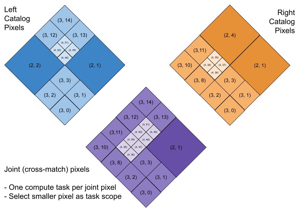
Catalogs have valuable metadata about their partitioning structure (e.g. the sky coverage and the order of the pixels at each point in the sky). LSDB takes advantage of this information for operations like joining/crossmatching to identify pairs of partitions that are spatially close to each other in the sky. Each core available to your distributed Dask client will process a pair of partitions at a time.

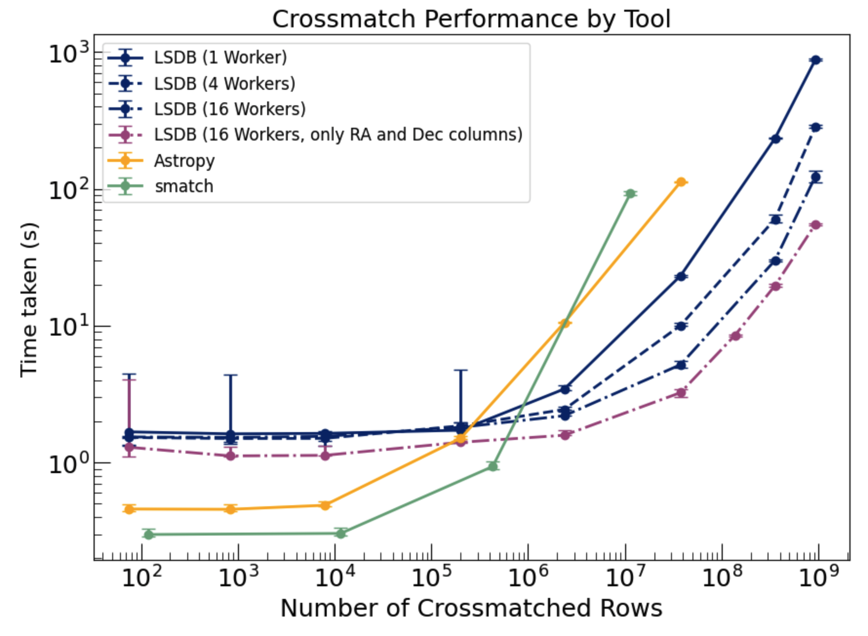
The benchmarking plot below demonstrates the performance of different methods forcross-matching using the nearest neighbor approach within 1 arcsecond. The LSDB approach (blue lines) shows superior scalability as the number of cross-matched objects increases, particularly when leveraging parallel workers (e.g., 4, 16 workers). In comparison, traditional methods become significantly slower as the dataset size grows. Additionally LSDB can also work on datasets that exceed the memory limits of the machine.

Export catalogs to disk

Once the analysis is complete we can export our results in the HATS format. To do so you would uncomment the line below. You need to provide a base directory path for your catalog and you should also provide a catalog name that expresses the nature of your data. You can load the saved catalog back via LSDB, or you can load the parquet files that are saved to disk with any other parquet reader of your choice.

# Export crossmatched data to disk
# _all_sky_object.to_hats(base_catalog_path="ztf_x_gaia", catalog_name="ztf_x_gaia")

Extra topics

Margin caches

Margins are catalogs that specify what objects, for each pixel, are within a certain distance of their borders. They allows us to crossmatch objects which might be just across the border, in the neighboring pixels, which you might miss if you only search among the objects in a given pixel.

In the image below we are trying to obtain the matches for the points in the “green” pixel. The closest match for the selected green object is in a different pixel. The closest green neighbor to this object is not even within the specified crossmatching radius (seen in dark green). This means that, without margin caches, this green object would simply not have a match, which is inaccurate!

Notice that your crossmatching distance, radius_arcsec, should not be larger than your margin cache radius. You can usually infer the margin cache radius from the catalog name, or look for it programatically.

ztf_object_full.margin.hc_structure.catalog_info.margin_threshold

10.0