Kernel-based Moving Object Detection (KBMOD) Demonstration

GitHub: http://github.com/dirac-institute/kbmod

In this notebook, we demonstrate how our shift-and-stack program KBMOD can search a set of images for a trans-Neptunian object (TNO) that is too faint to detect confidently in any one image. These images were acquired with the Vera C. Rubin Observatory Commissioning Camera (ComCam) as part of the Science Validation process. We made use of the SkyBot service to determine which solar system objects were in the ComCam data. We identified a single TNO, 2013 TA228, which we targeted to test our generalized LSST KBMOD search approach.

Note: The data are currently under embargo, so image data will not be included here; however, images will be shown during the live demo.

Initial Setup

show_embargoed = False  # show pixel data currently under Rubin embargo

# Load general libraries needed
from astropy.time import Time
from astropy.wcs import WCS
from astropy.coordinates import EarthLocation, SkyCoord
from astropy.table import Table
from astropy.table import conf
import astropy.units as u

import numpy as np

from datetime import datetime

from matplotlib import pyplot as plt

import glob

import os

os.environ["TF_CPP_MIN_LOG_LEVEL"] = "3"  # Suppress GPU logging

# Import the needed KBMOD components
import kbmod
from kbmod.configuration import SearchConfiguration
import kbmod.reprojection as reprojection
from kbmod.reprojection_utils import correct_parallax_geometrically_vectorized
from kbmod.filters.known_object_filters import KnownObjsMatcher
from kbmod.filters.stamp_filters import filter_stamps_by_cnn
from kbmod.results import Results
from kbmod.analysis.plotting import *
from kbmod.analysis.plotting import plot_ic_image_bounds, plot_wcs_on_sky
from kbmod.analysis.visualizer import Visualizer

# Import the LSST Butler interface for accessing ComCam data
import lsst.daf.butler as dafButler

# Confirm that a GPU is available and that at least 30 Gb of RAM is available
kbmod.search.validate_gpu(30 * 1024 * 1024 * 1024)

True

# Working directories
basedir = f"rubin-user/lincc_fw_kbmod_demo"  # Root directory for the demo.
workdir = f"{basedir}/20X20_patch250060"  # The subdirectory where images and other input and output files will be located

# The file contains the configuration parameters used for the KBMOD search.
kbmod_config_path = f"{workdir}/search_config_deep_20250122_39au_a.yaml"

# The KBMOD ImageCollection containing Butler-derived metadata.
full_comcam_ic_path = (
    f"{basedir}/LSSTComCam_runs_DRP_20241101_20241211_w_2024_50_DM-48128.collection"
)

# This is an ImageCollection, output by kbmod.ImageCollection
ic_path = f"{workdir}/tno_2013_TA228_ComCam_w50_20x20_patch250060_betterIDs.collection"

# Define the filename of the WorkUnit that combines the metadata from the ImageCollection and the image data from the Butler.
wu_filename = "tno_2013_TA228_ComCam_w50_20x20_patch110571_wu.fits"

# Reprojected (i.e., reflex-corrected) configuration.
repro_shard_dir = os.path.join(
    workdir, "repro"
)  # The directory to store the reprojected WorkUnit.
repro_workunit_filename = wu_filename + ".repro"

# Paths for results filtering and analysis
ml_model_path = f"{basedir}/kbmod_comcam_05.h5"  # the CNN model
skybot_table_path = f"/sdf/home/c/colinc/skytable.csv"  # solar system objects viewable in the ComCam fields found via SkyBot service

# Create any missing directories
for dirname in [basedir, workdir, repro_shard_dir]:
    os.makedirs(dirname, exist_ok=True)

Exploring the Rubin Solar System Science Validation Field

Here we load a KBMOD ImageCollection, a table of metadata derived (in this case) from LSST ComCam Butler Collection of difference image data and optimized for efficient analyses. The goal of this section is to visualize the on-sky availability of image data we can search.

comcam_ic = kbmod.ImageCollection.read(full_comcam_ic_path)
print(
    f'The full ComCam Butler contains {len(set(comcam_ic["visit"]))} science exposures.'
)

The full ComCam Butler contains 1943 science exposures.

Narrowing down the search area

Rubin observed an area of the sky (labeled “Rubin_SV_38_7”) near the plane of the solar system (ecliptic), where we are most likely to find TNOs.

ecliptic_comcam_field = "Rubin_SV_38_7"  # This is the label for the ecliptic field
ecliptic_ic = comcam_ic[comcam_ic["object"] == ecliptic_comcam_field]
print(
    f'There were {len(set(ecliptic_ic["visit"]))} exposures for {ecliptic_comcam_field}.'
)

There were 175 exposures for Rubin_SV_38_7.

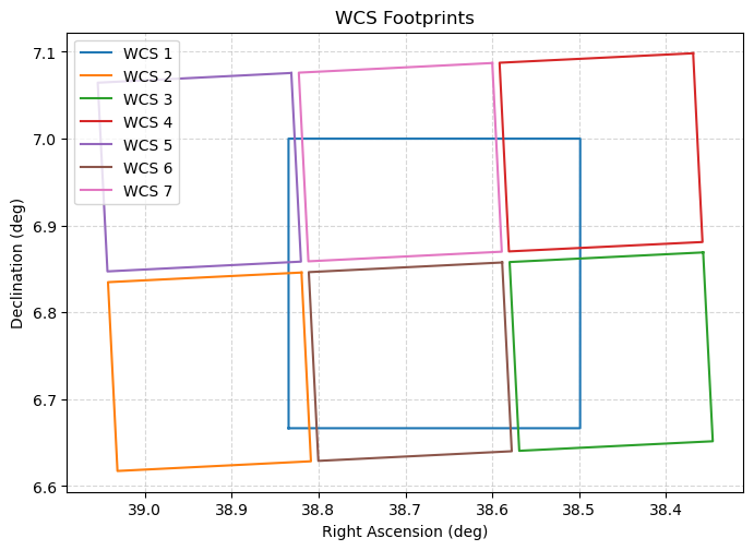
Next we visualize the on-sky area covered by the ecliptic ComCam observations.

_ = plot_ic_image_bounds(ecliptic_ic, lw=0.1)

Load the ImageCollection and generate WorkUnit

This ImageCollection is a collection of ComCam image metadata that overlaps with a 20’ X 20’ patch of the sky as generated by our Region Search toolset. We chose 20’ X 20’ patches as an optimal size to fit on the available GPU architecture. We use the ImageCollection to gather Butler-derived images into a KBMOD WorkUnit. Note that (at present) it takes roughly 4 seconds per image retrieval through the USDF Butler.

# Load the ImageCollection
ic = kbmod.ImageCollection.read(ic_path)
print(f"Read {len(ic)} rows from {ic_path}.")

Read 249 rows from rubin-user/lincc_fw_kbmod_demo/20X20_patch250060/tno_2013_TA228_ComCam_w50_20x20_patch250060_betterIDs.collection.

# Example row from the ImageCollection, trimmed to remove bulky columns (e.g., WCS)
display_ic = ic.data.copy()
display_ic.remove_columns(["wcs", "global_wcs", "config"])
display_ic[0]

Row index=0

dataId	std_idx	visit	detector	band	filter	mjd_start	mjd_mid	object	pointing_ra	pointing_dec	airmass	wcs_err	ra	dec	ra_bl	dec_bl	ra_tl	dec_tl	ra_tr	dec_tr	ra_br	dec_br	psfSigma	psfArea	nPsfStar	zeroPoint	skyBg	skyNoise	meanVar	OBSID	exposureTime	ext_idx	std_name	collection	datasetType	obs_lon	obs_lat	obs_elev	astromOffsetMean	astromOffsetStd	DIMM2SEE	global_wcs_pixel_shape_0	global_wcs_pixel_shape_1
str36	int64	int64	int64	str1	str4	float64	float64	str13	float64	float64	float64	float64	float64	float64	float64	float64	float64	float64	float64	float64	float64	float64	float64	float64	int64	float64	float64	float64	float64	str20	float64	int64	str18	str56	str28	float64	float64	float64	float64	float64	float64	int64	int64
615b2f69-ba41-4d4b-b29b-a807e7a3ac82	0	2024112600134	8	i	i_06	60641.08122699644	60641.08140639459	Rubin_SV_38_7	38.0653955028628	6.52826805904292	1.28850130948918	-3.090860900556436e-12	38.18728959931873	6.2575399328953285	38.13367905883207	6.407125257662862	38.03592432637463	6.206883852393906	38.24092893534934	6.107783069946998	38.33871170185693	6.30809586582424	2.1870157927318044	67.46518367993608	102	31.76327910494223	2581.0746131539345	52.993192583897475	2795.876509900088	CC_O_20241126_000134	30.0	0	ButlerStandardizer	LSSTComCam/runs/DRP/20241101_20241211/w_2024_50/DM-48128	goodSeeingDiff_differenceExp	-70.7494170285165	-30.2446389756252	2662.99616375123	nan	nan	0.0	6000	6000

%%time

wu = ic.toWorkUnit(
    search_config=SearchConfiguration.from_file(kbmod_config_path),
    butler=dafButler.Butler("/repo/embargo"),
)
wu.to_sharded_fits(wu_filename, workdir, overwrite=True)  # save the WorkUnit to disk
print(
    f"WorkUnit {wu_filename} contains {len(wu)} images, spanning {len(set(wu.get_all_obstimes()))} unique timestamps."
)

WorkUnit tno_2013_TA228_ComCam_w50_20x20_patch110571_wu.fits contains 249 images, spanning 57 unique timestamps.
CPU times: user 20min 2s, sys: 2min 33s, total: 22min 36s
Wall time: 28min 58s

Inspect ComCam images from the first exposure in the WorkUnit

Now that we have materialized our WorkUnit, we can access the data efficiently. Note the artifacts present in the image data example shown here.

first_visit_slices = wu.get_unique_obstimes_and_indices()[1][0]
first_wu_visit = wu.get_constituent_meta("visit")[0]

if show_embargoed:
    for visit_slice in first_visit_slices:
        im = wu.im_stack.get_single_image(visit_slice).get_science().image
        vmin, vmax = np.percentile(im, [1, 99])
        plt.imshow(im, cmap="gray", vmin=vmin, vmax=vmax)
        plt.colorbar(label="Pixel Value")
        plt.show()
        plt.close()
        break

Create reflex-corrected WCS for each image

Create new world coordinate system (WCS) elements for each image in the WorkUnit, correcting for the parallax imparted by Earth’s motion around the Sun for (as yet undiscovered) objects at 39 au.

# This is the target search distance in astronomical units for our reflex-correction and reprojection routines
target_search_dist = 39.0  # au

%%time

# Find the estimated barycentric distance (EBD) world coordinate system (WCS) for each image
ebd_per_image_wcs, geocentric_dists = kbmod.reprojection_utils.transform_wcses_to_ebd(
    [wu.get_wcs(i) for i in range(len(wu))],
    height=wu.get_wcs(0).array_shape[0],
    width=wu.get_wcs(0).array_shape[1],
    heliocentric_distance=target_search_dist,  # heliocentric reflex correction distance in au
    obstimes=Time(wu.get_all_obstimes(), format="mjd"),
    point_on_earth=EarthLocation.of_site("Rubin Observatory"),
    npoints=10,
)

# Store reflex-corrected WCSs and metadata in the WorkUnit.
wu.org_img_meta["ebd_wcs"] = ebd_per_image_wcs
wu.heliocentric_distance = target_search_dist
wu.org_img_meta["geocentric_distance"] = geocentric_dists

CPU times: user 38.6 s, sys: 715 ms, total: 39.3 s
Wall time: 40.5 s

Reprojecting images to common WCS

Here, we create mosaics from the input images and handle arbitrary image rotation. We built these features upon the extant AstroPy Reproject functionality.

%%time
common_wcs = WCS(ic.data["global_wcs"][0])
common_wcs.pixel_shape = (
    ic.data["global_wcs_pixel_shape_0"][0],
    ic.data["global_wcs_pixel_shape_1"][0],
)

reprojected_wu = reprojection.reproject_work_unit(
    wu,
    common_wcs,
    parallelize=True,
    frame="ebd",
    max_parallel_processes=16,
)
reprojected_wu.to_sharded_fits(repro_workunit_filename, repro_shard_dir, overwrite=True)

Reprojecting: 100%|██████████| 57/57 [42:41]

CPU times: user 29.4 s, sys: 2min 20s, total: 2min 50s
Wall time: 43min 46s

desired_slice = 0
chip_WCSs = []

for slice in wu.get_unique_obstimes_and_indices()[1][desired_slice]:
    chip_WCSs.append(ebd_per_image_wcs[slice])

if show_embargoed:
    im = reprojected_wu.im_stack.get_single_image(desired_slice).get_science().image
    vmin, vmax = np.percentile(im, [1, 99])
    plt.imshow(im, cmap="gray", vmin=vmin, vmax=vmax, origin="lower")
    plt.colorbar(label="Pixel Value")

_ = plot_wcs_on_sky([reprojected_wu.get_wcs(desired_slice)] + chip_WCSs)

Run the KBMOD search

Here we configure and execute a broad KBMOD search that reflects our general strategy for discovering distant solar system objects in LSST data.

# First, modify and update the KBMOD configuration based on the .yaml file.
config = kbmod.configuration.SearchConfiguration.from_file(kbmod_config_path)
timestamp = datetime.now().strftime("%Y%m%d_%H%M%S")
resultsdir = f"{workdir}/results_{timestamp}"
os.makedirs(resultsdir, exist_ok=True)

full_results_path = os.path.join(resultsdir, "full_results.ecsv")

settings = {
    "generator_config": {
        "name": "EclipticCenteredSearch",  # perform our search in relation to the plane of the solar system
        "velocities": [
            25,  # minimum velocity, in the units specified by velocity_units below
            225,  # maximum velocity, in the units specified by velocity_units below
            64,  # number of steps spanning the velocity search range
        ],
        "velocity_units": "pix / d",
        "angles": [
            90,  # minimum search angle w.r.t. the ecliptic, in the units specified by angle_units below
            -90,  # maximum search angle w.r.t. the ecliptic, in the units specified by angle_units below
            64,  # number of steps spanning the angle space to search
        ],
        "angle_units": "degree",
    },
    "result_filename": full_results_path,  # path to .ecsv results file
    "res_filepath": resultsdir,  # the directory to output any additional results
}
config.set_multiple(settings)

reprojected_wu.config = config

config.to_file(
    os.path.join(resultsdir, "search_config.yaml")
)  # save the configuration yaml for provenance

%%time

res = kbmod.run_search.SearchRunner().run_search_from_work_unit(reprojected_wu)
res.write_table(full_results_path)

print(
    f"Found {len(res)} results spanning {len(reprojected_wu)} unique timestamps/images."
)

WARNING:jax._src.xla_bridge:An NVIDIA GPU may be present on this machine, but a CUDA-enabled jaxlib is not installed. Falling back to cpu.

Found 157 results spanning 57 unique timestamps/images.
CPU times: user 31min 12s, sys: 5min 18s, total: 36min 30s
Wall time: 30min 55s

KBMOD-ML filtering of results with a prototype CNN

We are looking for very faint objects at a very low signal-to-noise ratio, and, consequently, many false positives are produced during the search phase. Here we employ a simple network trained on a limited set of ComCam data to filter out images unlikely to show a real minor planet.

Each row of the results table represents a trajectory, its associated likelihood, and provenance metadata.

%%time

filter_stamps_by_cnn(
    res,
    ml_model_path,
    coadd_type="mean",
)

res.filter_rows(res["cnn_class"])

CPU times: user 1.84 s, sys: 1.96 s, total: 3.8 s
Wall time: 9.76 s

Results length=22

x	y	vx	vy	likelihood	flux	obs_count	psi_curve	phi_curve	obs_valid	stamp	coadd_sum	coadd_mean	coadd_median	coadd_weighted	pred_x	pred_y	global_ra	global_dec	img_ra	img_dec	img_x	img_y	cnn_class
int64	int64	float64	float64	float64	float64	int64	float64[57]	float64[57]	bool[57]	float32[21,21]	float32[21,21]	float32[21,21]	float32[21,21]	float32[21,21]	float64[57]	float64[57]	float64[57]	float64[57]	float64[57]	float64[57]	float64[57]	float64[57]	bool
5806	4356	56.43665313720703	204.66281127929688	36.18541069178031	408.0334010176237	13	0.021866656839847565 .. 0.0	0.0007294111419469118 .. 0.0	True .. False	20.23334 .. -94.70616	20.23334 .. -94.70616	0.20920493 .. -11.737687	-0.892758 .. -15.635595	0.4706418 .. -13.5011215	5806.5 .. 6595.212314990027	4356.5 .. 7216.699368733327	38.509554174106526 .. 38.46534989502967	6.908724233093626 .. 7.0676054724718105	37.99950777072311 .. 37.65020753113546	6.548096974723788 .. 6.637261099587939	-3265.7342346515434 .. -4678.760098605894	-1234.9678896386515 .. -3509.434930227521	True
5699	4540	-90.18154907226562	-202.6667022705078	21.636266696267654	139.48144378247687	28	0.0 .. 0.0	0.0 .. 0.0	False .. False	-3.855865 .. 159.08072	-3.855865 .. 159.08072	-0.1676726 .. 5.853974	-0.2045532 .. 2.0483239	-0.34978858 .. 5.0418344	5699.5 .. 4439.196732808537	4540.5 .. 1708.1966114458473	38.51553881689849 .. 38.58609544699804	6.918948322922115 .. 6.761615447790551	38.00561554046287 .. 37.77376536820506	6.558564834967566 .. 6.325401982056455	-3249.8332376762755 .. -2203.885892032664	-1452.0794408411098 .. 1981.7598218750734	True
1949	5209	-17.98046875	224.28041076660156	21.454490490696276	352.73717113297073	8	0.20420870184898376 .. 0.0	0.0006917000864632428 .. 0.0	True .. False	0.77013946 .. -29.16818	0.77013946 .. -29.16818	-0.100083984 .. -3.322124	0.11093342 .. -2.8502007	1.5113386 .. -2.1484447	1949.5 .. 1698.2197354183827	5209.5 .. 8343.85882798692	38.72540442743863 .. 38.739494440757106	6.956135081307372 .. 7.130261575762976	38.22015755804006 .. 37.92941275832548	6.596832843939637 .. 6.701618950071004	-101.53375772224335 .. 237.1118383536974	-3745.320939526413 .. -4907.2114066174245	True
958	5536	-157.93850708007812	160.2511444091797	21.34441288926638	1402.2396725884832	8	0.11928845942020416 .. 0.0	5.621158197754994e-05 .. 0.0	True .. False	-63.087055 .. -18.010695	-63.087055 .. -18.010695	-8.205102 .. -1.4904785	-4.993581 .. -0.01013577	-5.1580286 .. -3.1463404	958.5 .. -1248.7188661214773	5536.5 .. 7776.038386152787	38.78087232587586 .. 38.90446999700032	6.974291552722317 .. 7.098661938523675	38.27685358452782 .. 38.097567883544286	6.615469142981776 .. 6.669664016320991	662.8313851602777 .. 3263.145364664731	-4489.756106036503 .. -4481.656509372213	True
5919	2932	-143.79998779296875	119.39411163330078	16.20137890938901	99.0629908946779	38	0.015175960026681423 .. 0.009721929207444191	0.0004723590100184083 .. 0.0004808444937225431	True .. True	-3.399155 .. -0.8875536	-3.399155 .. -0.8875536	-0.09186905 .. 0.21398003	-0.5983776 .. -1.1679907	-2.7276354 .. -0.015119868	5919.5 .. 3909.8694680123112	2932.5 .. 4601.054050388868	38.50325757649764 .. 38.615691293298	6.829611374939618 .. 6.922333551456416	37.993156529452705 .. 37.80364087396999	6.46713967359623 .. 6.489354554698109	-2731.2927110080623 .. -1816.8844973030682	125.06629170645658 .. -985.4264162302392	True
5903	1394	-33.183048248291016	-42.05690383911133	12.383961779984718	96.89468373950923	28	0.0011428374564275146 .. 0.0	0.0007491682772524655 .. 0.0	True .. False	-60.04982 .. 6.2468038	-60.04982 .. 6.2468038	-1.9789535 .. -0.057001058	-2.1704392 .. -0.34152177	-4.062559 .. 0.06314609	5903.5 .. 5439.760969644903	1394.5 .. 806.7472516643635	38.50418184716348 .. 38.530133755347784	6.744167646762159 .. 6.711522815700898	37.99419410776594 .. 37.71683460166332	6.379712676217073 .. 6.274229064564032	-2027.6290900309648 .. -3172.339575868223	1531.4937546277333 .. 2947.7501223352206	True
5713	2654	-102.30045318603516	175.0812530517578	14.35434272564229	89.73874839204488	25	0.03027910739183426 .. 0.0	0.0007080392097122967 .. 0.0	True .. False	35.526382 .. 93.54031	35.526382 .. 93.54031	-0.08953918 .. 2.0856016	-0.88798666 .. 1.7052162	-1.9852548 .. 1.5718077	5713.5 .. 4283.832881704974	2654.5 .. 5101.291805142831	38.51478862818741 .. 38.59475885899269	6.814170729998362 .. 6.9501217407191485	38.004963311537836 .. 37.782264709078994	6.451352113908676 .. 6.517660155848206	-2417.2839971276817 .. -2222.5865098258882	288.50252681047675 .. -1475.1252529908672	True
4199	2179	-92.6096420288086	-162.34791564941406	13.972461644419681	96.6801850409863	28	-0.023373544216156006 .. 0.0	0.0008316717576235533 .. 0.0	True .. False	0.49111068 .. 105.27103	0.49111068 .. 105.27103	1.1374611 .. 3.1722946	1.3948504 .. 1.136644	1.7147212 .. 2.049722	4199.5 .. 2905.2636997473783	2179.5 .. -89.34113900861666	38.59950149202201 .. 38.67190961436391	6.787800944826847 .. 6.661759310819151	38.091607480699444 .. 37.861367789270055	6.424455402650073 .. 6.223701323568043	-812.535497521165 .. -552.641993544044	47.92798777655954 .. 3730.401219749755	True
3703	1143	7.958179950714111	46.546810150146484	12.842587889491048	84.71877888998442	33	0.05382294952869415 .. 0.0	0.00012102875916752964 .. 0.0	True .. False	-81.15636 .. 44.054718	-81.15636 .. 44.054718	-2.5628412 .. 1.2438331	-0.13909239 .. 0.9206163	-0.145747 .. 1.3052158	3703.5 .. 3814.716987243648	1143.5 .. 1793.999991551061	38.627256266807585 .. 38.62103123669485	6.730248533702312 .. 6.766386792504737	38.12004764448969 .. 37.8093518064176	6.365593494038168 .. 6.330323158908446	107.06961222278667 .. -1574.3486950846996	778.1067934701987 .. 1863.0723171415098	True
...	...	...	...	...	...	...	...	...	...	...	...	...	...	...	...	...	...	...	...	...	...	...	...
5473	2588	-54.183082580566406	188.8077850341797	7.606332733909216	51.53387784276165	27	0.0 .. 0.00386595306918025	0.0 .. 0.0004649047623388469	False .. True	-67.465706 .. 10.961738	-67.465706 .. 10.961738	-0.9301708 .. 1.0347639	-0.9377326 .. -0.53472686	-1.8812326 .. -0.61405647	5473.5 .. 4716.28173633864	2588.5 .. 5227.122543055657	38.52821779098108 .. 38.57055477421673	6.810508082637383 .. 6.957108034076166	38.01869801614823 .. 37.75759181684762	6.447618023073037 .. 6.524745591460983	-2167.0219885572305 .. -2668.225825176851	241.83242704988822 .. -1581.1211864437057	True
4508	3928	-175.17662048339844	-108.30296325683594	9.387555670463884	56.3853515800497	38	0.0 .. 0.0	0.0 .. 0.0	False .. False	-35.88205 .. -106.83333	-35.88205 .. -106.83333	-1.5846661 .. -2.8771472	-0.58853585 .. -1.063135	0.2804402 .. -0.42563635	4508.5 .. 2060.3754179541675	3928.5 .. 2414.946730586437	38.58219652076092 .. 38.719181968432956	6.884964797791103 .. 6.800883103020223	38.07380806127428 .. 37.90929608400328	6.523859973135948 .. 6.365659378535414	-1880.1246743011186 .. 175.16516045383554	-1421.9133981668729 .. 1143.1109052471595	True
5602	3887	-74.19243621826172	35.255226135253906	12.075981370822346	70.38967159853745	37	0.014998147264122963 .. -0.0037089847028255463	0.0007270314963534474 .. 0.0004828212258871645	True .. True	-18.720833 .. 51.60132	-18.720833 .. 51.60132	-0.35166273 .. 1.0744153	-0.5335913 .. 0.095541105	-0.7444604 .. 0.35781348	5602.5 .. 4565.647442811825	3887.5 .. 4380.198086703182	38.52097825165853 .. 38.57899400864406	6.8826723955090765 .. 6.910058502960804	38.01121708813902 .. 37.76627289940263	6.521451523437192 .. 6.476776495309364	-2867.810380870024 .. -2471.328153343442	-894.8503059433689 .. -727.5676770624968	True
3047	5592	-140.11123657226562	142.16282653808594	11.804372341774288	413.7793703361184	8	0.0703236535191536 .. 0.0	0.00020506029250100255 .. 0.0	True .. False	12.979774 .. 9.6973715	12.979774 .. 9.6973715	1.5654112 .. 1.3853388	2.277811 .. -1.5026748	2.846086 .. 1.7435354	3047.5 .. 1089.4204256431597	5592.5 .. 7579.250910827104	38.66395212716434 .. 38.773570180847905	6.977416355193158 .. 7.087777832534702	38.157299601457666 .. 37.964209236769456	6.6185459939676 .. 6.658346189215684	-1282.6928488196675 .. 895.2788987439203	-3606.424934177934 .. -4160.1464381953865	True
5663	5586	-101.15679931640625	113.43049621582031	7.816344372545343	127.73265703813134	11	0.03316514566540718 .. 0.0	0.00046595142339356244 .. 0.0	True .. False	-15.995832 .. -16.329336	-15.995832 .. -16.329336	-0.84943336 .. -1.6618574	-3.3020778 .. -2.7392411	-1.0653406 .. -1.4115922	5663.5 .. 4249.815648947911	5586.5 .. 7171.71145900245	38.51753534434539 .. 38.59664583911996	6.977059630723896 .. 7.065144149051785	38.00759246876685 .. 37.78398297682736	6.618028916488452 .. 6.634969077940713	-3685.958698169858 .. -2295.1759955894354	-2430.559867137835 .. -3583.0576676185215	True
3407	743	-107.7586441040039	-111.63469696044922	8.601848087207001	64.26481555737193	21	0.0 .. 0.0	0.0 .. 0.0	False .. False	0.1323638 .. 20.150505	0.1323638 .. 20.150505	-1.4653327 .. 0.90531445	0.38149494 .. 0.62079966	-0.03282839 .. 0.5452787	3407.5 .. 1901.5536880380037	743.5 .. -816.6148434303382	38.64381584767605 .. 38.72804486704114	6.70802744892924 .. 6.6213519325659265	38.13700300973308 .. 37.918630562064976	6.342872573334869 .. 6.182579642832663	558.0425046661936 .. 504.70770388942793	1013.1909687166695 .. 4418.382194508643	True
4050	5382	-38.51970672607422	212.00523376464844	8.057156627446933	262.0833303873792	7	0.11224542558193207 .. 0.0	0.00019485079974401742 .. 0.0	True .. False	-4.9571695 .. -4.3161826	-4.9571695 .. -4.3161826	0.034389496 .. -0.6626034	1.4952997 .. -1.4586768	1.703118 .. -0.9431027	4050.5 .. 3512.1802135520393	5382.5 .. 8345.311035339024	38.60781578793283 .. 38.63793483779249	6.965746125844088 .. 7.130347065226834	38.0999141024019 .. 37.825934020815865	6.606546121722411 .. 6.701536360290903	-2110.8363892465536 .. -1606.399658119522	-2964.408916516583 .. -4815.316658730674	True
332	2583	-38.88623809814453	113.77635955810547	7.962845775059378	60.717427452486156	22	0.0 .. 0.0	0.0 .. 0.0	False .. False	16.933348 .. 33.72195	16.933348 .. 33.72195	1.1358886 .. -0.102291495	0.8899715 .. 0.16415961	0.13089246 .. 0.46824718	332.5 .. -210.9421278858773	2583.5 .. 4173.544961029948	38.815857855481525 .. 38.84629655019088	6.810227130746243 .. 6.8985522263938925	38.31280468662382 .. 38.03864542313396	6.447620536128645 .. 6.465472923089018	2560.2443879652087 .. 2392.675141056863	-2053.728039251649 .. -761.2647513842826	True
2959	1306	-66.56809997558594	-201.59527587890625	7.380237638756289	53.64604529404078	26	0.041234731674194336 .. 0.0	0.0007394053973257542 .. 0.0	True .. False	-60.94166 .. 82.30436	-60.94166 .. 82.30436	0.5744564 .. 1.596767	0.8632641 .. 0.9292253	0.14690402 .. 0.21601103	2959.5 .. 2029.1989045649448	1306.5 .. -1510.8300132264726	38.66887637641392 .. 38.72090153116393	6.7393056350010845 .. 6.58278589520659	38.16259341143577 .. 37.911416591940124	6.374902579352502 .. 6.143237949601344	717.8714769836095 .. 411.3148084089031	295.49540366702104 .. 5129.764121475218	True
2226	5990	37.91838836669922	221.7818603515625	8.044575738792933	190.08875031504928	8	0.059007223695516586 .. 0.0	0.0003396226966287941 .. 0.0	True .. False	14.603372 .. 0.0	14.603372 .. 0.0	1.739654 .. 0.0	2.72528 .. 0.0	2.121596 .. 0.0	2226.5 .. 2756.4162548970085	5990.5 .. 9089.941139349823	38.709905396104325 .. 38.68024957261137	6.999525338300865 .. 7.171714818524412	38.20426195416528 .. 37.86897309176125	6.64121717538698 .. 6.74379783599378	-706.2963534796628 .. -876.7464955274651	-4340.107521270118 .. -5612.347098917529	True

Visualize Results

Here we visualize results in the form of co-added image cutouts. For each row in the results table, we (1) generate a combined co-added image cutout that spans all results above the prescribed likelihood threshold, and (2) provide daily co-added cutouts.

if show_embargoed:
    res.table["stamp"] = res.table[
        "coadd_sum"
    ]  # We store the combined stamps in the results table.
    viz = Visualizer(
        reprojected_wu.im_stack, res
    )  # The image data are derived from the reprojected WorkUnit.
    viz.generate_all_stamps(radius=config["stamp_radius"])
    viz.count_num_days()  # This feature enables the daily image co-addition.

    for res_idx in range(10):  # first 10 results
        viz.plot_daily_coadds(res_idx)

Matching to known objects

For testing and validation in Rubin data we will make use of known small solar system bodies (e.g., TNOs) we previously identified in ComCam data with SkyBot. In the future we will make use of Rubin’s MPCSky routine to greatly optimize this process.

skytable = Table.read(skybot_table_path)
print(f"Read {skybot_table_path}. There are {len(skytable)} rows.")

Read /sdf/home/c/colinc/skytable.csv. There are 9544 rows.

known_objs_matcher = KnownObjsMatcher(
    skytable,
    np.array(reprojected_wu.get_all_obstimes()),
    matcher_name="known_matcher",
    sep_thresh=5.0,  # Observations must be within 5 arcsecs.
    time_thresh_s=30,  # Observations must match within 30 seconds.
    name_col="Name",
    ra_col=f"ra_{target_search_dist}",
    dec_col=f"dec_{target_search_dist}",
    mjd_col="mjd_mid",
)

# Carry out initial matching to known objects and populate the matches column.
known_objs_matcher.match(res, reprojected_wu.wcs)

# Filter the matches down to results with at least 10 observations.
min_obs = 10
known_objs_matcher.match_on_min_obs(res, min_obs)

matched_col_name = known_objs_matcher.match_min_obs_col(min_obs)

known_tno_results = []
for res_idx in range(len(res)):
    my_matches = res[res_idx][matched_col_name]
    if len(my_matches) >= 1:
        print(f"Result {res_idx} matched to objects: {my_matches}")
        if "2013 TA228" in my_matches:
            known_tno_results.append(res_idx)
        if show_embargoed:
            viz.plot_daily_coadds(res_idx)

Result 14 matched to objects: {'2013 TA228'}

Here we plot our KBMOD TNO trajectory against the cached SkyBot ephemeris results.

tnotable = skytable[skytable["Name"] == "2013 TA228"]
tnotable.sort("mjd_mid")

tno_res_idx = known_tno_results[0]

plt.plot(res[tno_res_idx]["global_ra"], res[tno_res_idx]["global_dec"], zorder=1)
for i, day_obs in enumerate(set(tnotable["day_obs"])):
    tno_day_table = tnotable[tnotable["day_obs"] == day_obs]
    plt.scatter(
        tno_day_table[f"ra_{target_search_dist}"],
        tno_day_table[f"dec_{target_search_dist}"],
        label=f"{day_obs}",
        marker=f"${i}$",
    )
_ = plt.legend()

Refine candidate trajectory with pencil search

Here we carry out a search for the TNO using a finer grid of candidate velocities derived from the initial KBMOD search. We use the KBMOD VelocityGridSearch method, which operates in pixel space instead of searching for angles centered around the ecliptic.

%%time

# First, modify and update the KBMOD configuration for the pencil search.
resultsdir = f"{workdir}/results_pencil_{timestamp}"
os.makedirs(resultsdir, exist_ok=True)

full_results_path = os.path.join(resultsdir, "full_results.ecsv")

settings = {
    "generator_config": {
        "name": "VelocityGridSearch",  # perform our search in relation to pixel/velocity space.
        "min_vx": int(res[tno_res_idx]["vx"]) - 2,
        "max_vx": int(res[tno_res_idx]["vx"]) + 2,
        "min_vy": int(res[tno_res_idx]["vy"]) - 2,
        "max_vy": int(res[tno_res_idx]["vy"]) + 2,
        "vx_steps": 20,
        "vy_steps": 20,
    },
    "result_filename": full_results_path,  # path to .ecsv results file
    "res_filepath": resultsdir,  # the directory to output any additional results
}
config.set_multiple(settings)

reprojected_wu.config = config

config.to_file(
    os.path.join(resultsdir, "search_config.yaml")
)  # save the configuration yaml for provenance

pencil_res = kbmod.run_search.SearchRunner().run_search_from_work_unit(reprojected_wu)

print(
    f"Found {len(pencil_res)} results from the pencil search for initial result {tno_res_idx}."
)

Found 22 results from the pencil search for initial result 14.
CPU times: user 1min 59s, sys: 29.4 s, total: 2min 29s
Wall time: 1min 45s

Matching against known objects to recover the TNO

Once again we match the search results against known objects, this time with the output from the pencil search. We then display the combined co-added images and daily cutouts for both the updated search result with the initial result to facilitate comparison. The results from the pencil search (result 9 below) indicate a better match to the object’s actual trajectory with the object appearing closer to the center of each cutout.

# Carry out initial matching to known objects and populate the matches column.
known_objs_matcher.match(pencil_res, reprojected_wu.wcs)
known_objs_matcher.match_on_min_obs(pencil_res, min_obs)

# Instantiate a KBMOD Vizualizer for the pencil search.
pencil_res.table["stamp"] = pencil_res.table[
    "coadd_sum"
]  # Store combined stamps in the results table.
pencil_viz = Visualizer(
    reprojected_wu.im_stack, pencil_res
)  # Image data are derived from the reprojected WorkUnit.
pencil_viz.generate_all_stamps(radius=config["stamp_radius"])
pencil_viz.count_num_days()  # Enable the daily image co-addition.

# Show the cutouts from our pencil search.
for res_idx in range(len(pencil_res)):
    my_matches = pencil_res[res_idx][matched_col_name]
    if len(my_matches) >= 1:
        print(f"Result {res_idx} matched to objects: {my_matches}")
        if show_embargoed:
            pencil_viz.plot_daily_coadds(res_idx)

# Display the initial known TNO result from the earlier search for comparison.
if show_embargoed:
    viz.plot_daily_coadds(tno_res_idx)

Result 11 matched to objects: {'2013 TA228'}

Next Steps

We next send results for orbit fitting; the upcoming selected incubator will help automate and optimize this process.

Summary & Key Takeaways

• KBMOD represents a novel way of working with Rubin images.

• KBMOD will lead to software facilitating scalable image science.

• Unique in LINCC Frameworks, KBMOD directly produces discoveries.

• Our work has demonstrated how KBMOD facilitates probing two magnitudes fainter.

  • This effectively transforms the 6.7 m Rubin into a 16 m telescope in terms of TNO discovery.

  • This will enhance the LSST discovery of TNOs by a factor of about 5X.

• KBMOD has proven success with multiple surveys (e.g., DEEP, KLASSI).

• KBMOD works with Rubin ComCam and ready for LSSTCam.

  • New: spanning multiple nights, filters, and rotation angles

  • We successfully recovered one TNO (as shown in this notebook) and one Jupiter Trojan in ComCam data.

• KBMOD is capable of LSST-scale deployment.