RAIL Demonstration with HSC dataset

This notebook demonstrates how RAIL can be used to apply different models and evaluation metrics. It uses the publically available HSC Y3 dataset.

RAIL wraps a variety of estimation models, simulation effects, and evaluation metrics so as to allow users to explore the space of solutions without having to learn numerous software packages. For example, the rail.estimation subpackage contains infrastructure to run multiple production-level photo-z codes. There is a minimal superclass that sets up some file paths and variable names. Each specific photo-z code resides in a subclass in rail.estimation.algos with algorithm-specific setup variables.

More extensive documentation is available on Read the Docs here: https://rail-hub.readthedocs.io/en/latest/

import os
import matplotlib.pyplot as plt
import numpy as np

%matplotlib inline
import warnings

warnings.filterwarnings("ignore")

import rail
import qp
from rail.core.data import TableHandle
from rail.core.stage import RailStage

Setup

RAIL is designed to run in both at-scale environments and local environments like Jupyter Notebooks.

To support production runs in a large environment, RAIL uses `ceci <LSSTDESC/ceci>`__ as a back-end for pipelines of RAIL stages run at the command line. To run locally, we use the DataStore object, which is a workaround to enable ceci to interact with data files in an interactive notebook environment. See the Golden Spike end-to-end demo notebook for more details on the DataStore.

We’ll start by setting up the DataStore. We load the data into the TableHandle with the DataStore.read_file().

DS = RailStage.data_store
DS.__class__.allow_overwrite = True

trainFile = "./data/dered_pdr3_wide_train_curated.pq"
testFile = "./data/dered_pdr3_wide_test_curated.pq"

training_data = DS.read_file("training_data", TableHandle, trainFile)
test_data = DS.read_file("test_data", TableHandle, testFile)

Set common parameters

We start configuring RAIL by setting parameters that are common to all stages. These include: the name of the bands, the reference band, the name of the magnitude error, and the magnitude limit. We also ask all estimation stages to compute mode and median as point estimate by calculated_point_estimates = ['zmode', 'zmedian']

The common_params streamlines running multiple algorithms.

from rail.core import common_params

common_params.set_param_defaults(
    mag_limits={
        "g_HSCMag": 27.8,
        "r_HSCMag": 27.1,
        "i_HSCMag": 26.6,
        "z_HSCMag": 26.6,
        "y_HSCMag": 25.6,
    },
    bands=[f"{band}_HSCMag" for band in "grizy"],
    ref_band="i_HSCMag",
    err_bands=[f"{band}_HSCMagErr" for band in "grizy"],
    calculated_point_estimates=["zmode", "zmedian"],
)

Training and applying a model

Models for photo-z estimators are trained using a pipeline stage called “inform”, which is informing the model about the data. This stage is carried out by an object known as an “informer” which does the actual training.

A corresponding stage, called the estimate stage, applies the trained model to new data points. Like the inform stage, the estimate stage uses an estimator object to perform the actual computation.

By breaking the flow into two stages, it allows users to skip any work that is unnecessary for their usecase. For example, if the user only wants to apply a pre-trained model, they can load it and apply the estimat estage directly.

Below we show how we can train a simple model using the infrastructure for the inform and estimate operations.

A simple k-NN model

Each photo-z algorithm has code-specific parameters necessary to initialize the code. These values can be input on the command line, or passed in via a dictionary.

Let’s start with a very simple demonstration using k_nearneigh, a RAIL wrapper around sklearn’s nearest neighbor (NN) method. It calculates a normalized weight for the K nearest neighbors based on their distance and makes a PDF as a sum of K Gaussians, each at the redshift of the training galaxy with amplitude based on the distance weight, and a Gaussian width set by the user. This is a toy model estimator, but it performs very well for representative data sets. There are configuration parameters for the names of columns, random seeds, etc. in KNearNeighEstimator with best-guess sensible defaults based on preliminary experimentation in DESC.

See the KNearNeigh code for more details, but here is a minimal settings to run:

knn_dict = dict(
    zmin=0.0,
    zmax=3.0,
    nzbins=301,
    trainfrac=0.75,
    sigma_grid_min=0.01,
    sigma_grid_max=0.07,
    ngrid_sigma=10,
    nneigh_min=3,
    nneigh_max=7,
    hdf5_groupname="",
)

Training

We create the knn informer (the object that will learn the model by ingesting the data) by feeding the configuration to RAIL’s the make_stage function. The name is specified for ceci to recognize the stage.

from rail.estimation.algos.k_nearneigh import KNearNeighInformer, KNearNeighEstimator

knn_informer = KNearNeighInformer.make_stage(
    name="inform_KNN",
    model="./model/demo_knn.pkl",
    **knn_dict
)

The inform step trains the model on the data. In the case of KNearNeighInformer, the stage finds the best fit parameters for the knn.

%%time
knn_informer.inform(training_data)

split into 15000 training and 5000 validation samples
finding best fit sigma and NNeigh...



best fit values are sigma=0.023333333333333334 and numneigh=7



Inserting handle into data store.  model_inform_KNN: model/inprogress_demo_knn.pkl, inform_KNN
CPU times: user 21.9 s, sys: 3.34 s, total: 25.3 s
Wall time: 25.3 s

<rail.core.data.ModelHandle at 0x1486ba784850>

Predicting

We make the knn estimator stage using the same configurations as we did for the informer stage.

knn_estimator = KNearNeighEstimator.make_stage(
    name="estimate_KNN",
    model="./model/demo_knn.pkl",
    output="./output/knn_output.hdf5",
    **knn_dict
)

We then run the estimate function to estimate the photo-z for the test_data

%%time

results_knn = knn_estimator.estimate(test_data)

Inserting handle into data store.  model: ./model/demo_knn.pkl, estimate_KNN
Process 0 running estimator on chunk 0 - 10000
Process 0 estimating PZ PDF for rows 0 - 10,000
Inserting handle into data store.  output_estimate_KNN: output/inprogress_knn_output.hdf5, estimate_KNN
Process 0 running estimator on chunk 10000 - 20000
Process 0 estimating PZ PDF for rows 10,000 - 20,000
CPU times: user 4.6 s, sys: 561 ms, total: 5.16 s
Wall time: 5.19 s

The results_knn object now holds the results of the estimation step. We can extract both the mode and median of the estimated photo-z and plot them.

zmode_knn = results_knn().ancil["zmode"].flatten()
zmedian_knn = results_knn().ancil["zmedian"].flatten()

plt.figure(figsize=(8, 8))
# plt.scatter(test_data()['redshift'],zmode_knn,s=1,label='KNN mode')
plt.scatter(test_data()["redshift"], zmedian_knn, s=1, label="KNN mode", c="k")

plt.plot([0, 4], [0, 4], "r--", alpha=0.7)

plt.xlim(0, 3)
plt.ylim(0, 3)
plt.xlabel("Spectroscopic z")
plt.ylabel("k-NN photo-z Mode")

Text(0, 0.5, 'k-NN photo-z Mode')

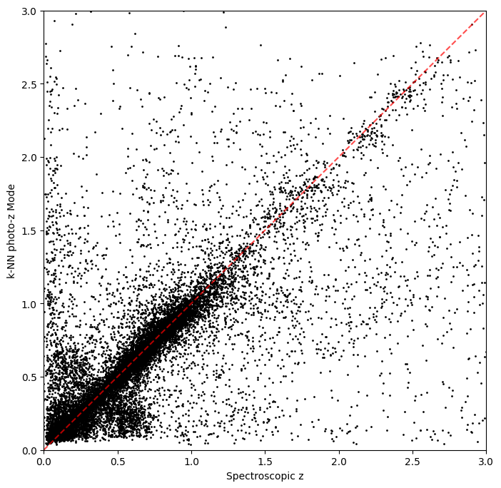
Not bad, given our very simple estimator!

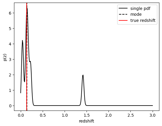
Internally RAIL makes use of the qp package to wrap different representations of statistical distributions and make them interoperable. In the example above KNearNeigh is storing each PDF as a Gaussian mixture model where each PDF is represented by a set of N Gaussians for each galaxy. We can evaluate these PDFs on a set of grid points with the built-in .pdf method.

Let’s pick a single galaxy from our sample and evaluate and plot the PDF, the mode, and true redshift:

zgrid = np.linspace(0, 3.0, 301)
galid = 1024
single_gal = np.squeeze(results_knn()[galid].pdf(zgrid))
single_zmode = zmode_knn[galid]
truez = np.array(test_data()["redshift"])[galid]

plt.plot(zgrid, single_gal, color="k", label="single pdf")
plt.axvline(single_zmode, color="k", ls="--", label="mode")
plt.axvline(truez, color="r", label="true redshift")
plt.legend(loc="upper right")
plt.xlabel("redshift")
plt.ylabel("p(z)")

Text(0, 0.5, 'p(z)')

FlexZBoost

The key advantage of RAIL is that is provides the same interface for a range of models. Let’s examine how the same analysis would be performed using the FlexZBoostEstimator estimator.

FlexZBoost Package

FlexZBoost is available in the rail_flexzboost repo and can be installed with

pip install pz-rail-flexzboost

on the command line or from source. Once installed, it will function the same as any of the other estimators included in the primary rail repo.

FlexZBoostEstimator approximates the conditional density estimate for each PDF with a set of weights on a set of basis functions. This can save space relative to a gridded parameterization, but it also leads to residual “bumps” in the PDF intrinsic to the underlying cosine or fourier parameterization. For this reason, FlexZBoostEstimator has a post-processing stage where it “trims” (i.e. sets to zero) any small peaks, or “bumps”, below a certain bump_thresh threshold.

One of the dominant features seen in our PhotoZDC1 analysis of multiple photo-z codes (Schmidt, Malz et al. 2020) was that photo-z estimates were often, in general, overconfident or underconfident in their overall uncertainty in PDFs. To remedy this, FlexZBoostEstimator has an additional post-processing step where it applies a “sharpening” parameter sharpen that modulates the width of the PDFs according to a power law.

A portion of the training data is held in reserve to determine best-fit values for both bump_thresh and sharpening, which we currently find by simply calculating the CDE loss for a grid of bump_thresh and sharpening values; once those values are set FlexZBoost will re-train its density estimate model with the full dataset. A more sophisticated hyperparameter fitting procedure may be implemented in the future.

We’ll start with a dictionary of setup parameters for FlexZBoostEstimator, just as we had for the k-nearest neighbor estimator. Some of the parameters are the same as in k-nearest neighbor above, zmin, zmax, nzbins. However, FlexZBoostEstimator performs a more in depth training and as such has more input parameters to control its behavior. These parameters are:

• basis_system: which basis system to use in the density estimate. The default is cosine but fourier is also an option

• max_basis: the maximum number of basis functions parameters to use for PDFs

• regression_params: a dictionary of options fed to xgboost that control the maximum depth and the objective function. An update in xgboost means that objective should now be set to reg:squarederror for proper functioning.

• trainfrac: The fraction of the training data to use for training the density estimate. The remaining galaxies will be used for validation of bump_thresh and sharpening.

• bumpmin: the minimum value to test in the bump_thresh grid

• bumpmax: the maximum value to test in the bump_thresh grid

• nbump: how many points to test in the bump_thresh grid

• sharpmin, sharpmax, nsharp: same as equivalent bump_thresh params, but for sharpening parameter

fz_dict = dict(
    zmin=0.0,
    zmax=4.0,
    nzbins=401,
    trainfrac=0.75,
    bumpmin=0.02,
    bumpmax=0.35,
    nbump=20,
    sharpmin=0.7,
    sharpmax=2.1,
    nsharp=15,
    max_basis=35,
    basis_system="cosine",
    hdf5_groupname="",
    regression_params={"max_depth": 8, "objective": "reg:squarederror"},
)
fz_modelfile = "model/demo_FZB_model.pkl"

Training FlexZBoost

As with the knn model, we create the inform stage of flexzboost:

from rail.estimation.algos.flexzboost import FlexZBoostInformer, FlexZBoostEstimator

fzb_informer = FlexZBoostInformer.make_stage(
    name="inform_fzboost",
    model=fz_modelfile,
    **fz_dict
)

FlexZBoostInformer operates on the training set and writes a file containing the estimation model. FlexZBoost uses xgboost to determine a conditional density estimate model, and also fits the bump_thresh and sharpen parameters described above.

FlexZBoost is a bit more sophisticated than the earlier k-nearest neighbor estimator, so it will take a bit longer to train, but not drastically so, still under a minute on a semi-new laptop. We specified the name of the model file, demo_FZB_model.pkl, which will store our trained model for use with the estimation stage.

%%time
fzb_informer.inform(training_data)

stacking some data...
read in training data
fit the model...
finding best bump thresh...
finding best sharpen parameter...
Retraining with full training set...
Inserting handle into data store.  model_inform_fzboost: model/inprogress_demo_FZB_model.pkl, inform_fzboost
CPU times: user 1min 41s, sys: 20.5 s, total: 2min 1s
Wall time: 2min 14s

<rail.core.data.ModelHandle at 0x1487101d4f50>

Predicting with FlexZBoost

Similar to the k-NN step, we now initialize the estimation stage of the FlexZBoost estimator. We directly take the model data from the informer stage fzb_informer. The output path is specified by output.

%%time
fzb_estimator = FlexZBoostEstimator.make_stage(
    name="fzboost",
    hdf5_groupname="photometry",
    model=fzb_informer.get_handle("model"),
    output="./output/output_fzboost.hdf5",
)

CPU times: user 135 µs, sys: 27 µs, total: 162 µs
Wall time: 167 µs

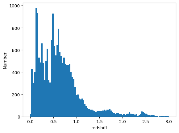
The results_fzb object now holds the results of the estimation step using FlexZBoost. We can extract both the mode and median of the estimated photo-z and plot them.

%%time
results_fzb = fzb_estimator.estimate(test_data)

Process 0 running estimator on chunk 0 - 10000
Process 0 estimating PZ PDF for rows 0 - 10,000
Inserting handle into data store.  output_fzboost: output/inprogress_output_fzboost.hdf5, fzboost
Process 0 running estimator on chunk 10000 - 20000
Process 0 estimating PZ PDF for rows 10,000 - 20,000
CPU times: user 13.3 s, sys: 1.39 s, total: 14.7 s
Wall time: 13.7 s

fz_medians = results_fzb().ancil["zmedian"].flatten()
fz_modes = results_fzb().ancil["zmode"].flatten()

plt.hist(fz_medians, bins=np.linspace(-0.005, 3.005, 101))
plt.xlabel("redshift")
plt.ylabel("Number")

Text(0, 0.5, 'Number')

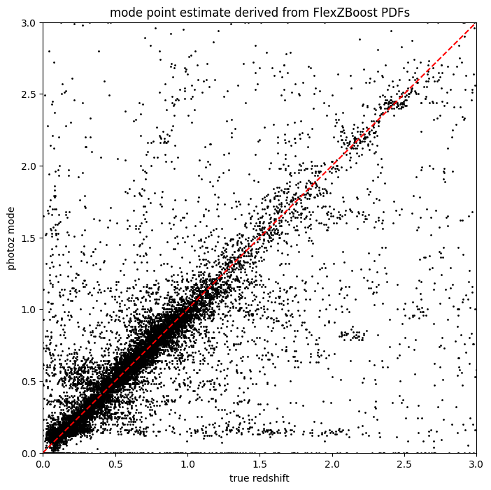
plt.figure(figsize=(8, 8))
plt.scatter(test_data()["redshift"], fz_modes, s=1, c="k")
plt.plot([0, 3], [0, 3], "r--")
plt.xlim(0, 3)
plt.ylim(0, 3)
plt.xlabel("true redshift")
plt.ylabel("photoz mode")
plt.title("mode point estimate derived from FlexZBoost PDFs")

Text(0.5, 1.0, 'mode point estimate derived from FlexZBoost PDFs')

BPZ

Finally let’s consider a third model for photo-z estimation: BPZ. (Benitez (2000))

from rail.utils.path_utils import RAILDIR
from rail.core.data import ModelHandle
from rail.estimation.algos.bpz_lite import BPZliteInformer, BPZliteEstimator

Running BPZliteEstimator with a pre-existing model

BPZ is a template-fitting code that works by calculating the chi^2 value for observed photometry and errors compared with a grid of theoretical photometric fluxes generated from a set of template SEDs at each of a grid of redshift values. These chi^2 values are converted to likelihoods. If desired, a Bayesian prior can be applied that parameterizes the expected distribution of galaxies in terms of both probability of a “broad” SED type as a function of apparent magnitude, and the probability of a galaxy being at a certain redshift given broad SED type and apparent magnitude. The product of this prior and the likelihoods is then summed over the SED types to return a marginalized posterior PDF, or p(z) for each galaxy. If the config option no_prior is set to True, then no prior is applied, and BPZliteEstimator will return a likelihood for each galaxy rather than a posterior.

We need to set up a RAIL stage for the default run of BPZ, including specifying the location of the model pickle file, which is located included in the rail_base package and can be found relative to RAILDIR at rail/examples_data/estimation_data/data/COSMOS31_HDFN_prior.pkl.

cosmospriorfile = os.path.join(
    RAILDIR, "rail/examples_data/estimation_data/data/COSMOS31_HDFN_prior.pkl"
)
cosmosprior = DS.read_file("cosmos_prior", ModelHandle, cosmospriorfile)
sedfile = os.path.join(
    RAILDIR, "rail/examples_data/estimation_data/data/SED/COSMOS_seds.list"
)
hsc_config = "/hildafs/projects/phy200017p/ztq1996/ztq1996/RAIL/rail_bpz/src/rail/examples_data/estimation_data/configs/bpz_hsc.columns"
filter_path = RAILDIR + "/rail/examples_data/estimation_data/data/FILTER"

bpz_dict = dict(
    output="output/bpz_results_cosmos_matched.hdf5",
    prior_band="i_cModelMag",
    no_prior=False,
    spectra_file=sedfile,
    zp_errors=[0.1] * 5,
    columns_file=hsc_config,
)

bpz_estimator = BPZliteEstimator.make_stage(
    name="bpz_def_prior", model=cosmosprior, **bpz_dict
)

The estimate will perform template fitting to the galaxy dataset

bpz_estimator.estimate(training_data)

Process 0 running estimator on chunk 0 - 10000
Inserting handle into data store.  output_bpz_def_prior: output/inprogress_bpz_results_cosmos_matched.hdf5, bpz_def_prior
Process 0 running estimator on chunk 10000 - 20000

<rail.core.data.QPHandle at 0x1486b97b36d0>

results_bpz = qp.read("./output/bpz_results_cosmos_matched.hdf5")
sz = training_data()["redshift"]

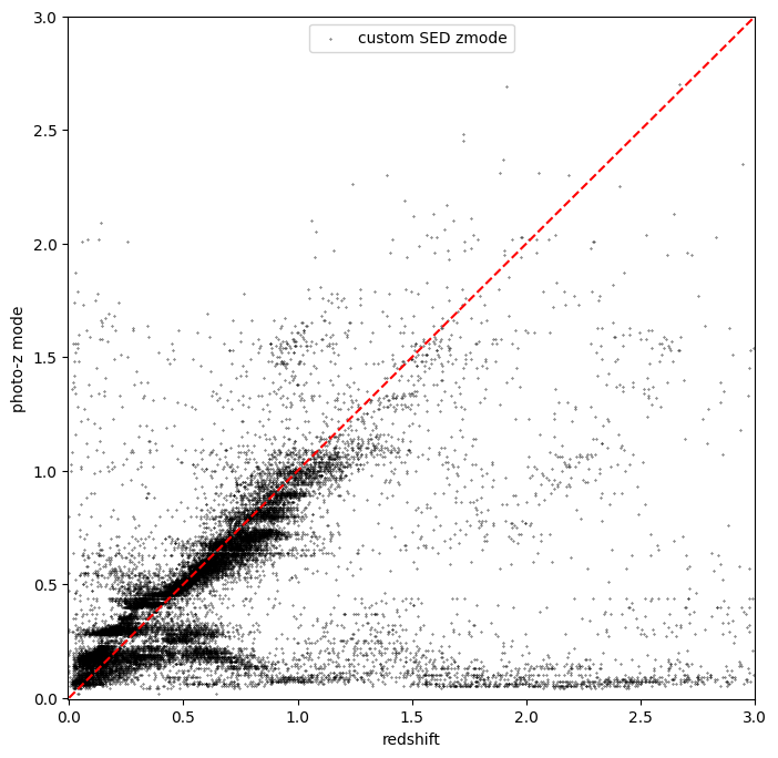
Make a plot to show the BPZ mode vs. spec-z

plt.figure(figsize=(8, 8))
plt.scatter(
    sz, results_bpz.ancil["zmode"].flatten(), s=0.1, c="k", label="custom SED zmode"
)
plt.plot([0, 3], [0, 3], "r--")
plt.xlabel("redshift")
plt.ylabel("photo-z mode")
plt.legend(loc="upper center", fontsize=10)
plt.xlim(-0.005, 3)
plt.ylim(-0.005, 3)

(-0.005, 3.0)

Evaluation

One of the major benefits of RAIL is it allows the user to evaluate various models against ground truth data, enabling researchers to determine which model will work well for their specific use case.

In this section we demonstrate the application of the metrics scripts to be used on the photo-z PDF catalogs produced by the PZ working group. The first implementation of the evaluation module is based on the refactoring of the code used in Schmidt et al. 2020, available on Github repository PZDC1paper.

import tables_io
import pandas as pd

from rail.evaluation.dist_to_dist_evaluator import DistToDistEvaluator
from rail.evaluation.dist_to_point_evaluator import DistToPointEvaluator
from rail.evaluation.point_to_point_evaluator import PointToPointEvaluator

# from rail.evaluation.single_evaluator import SingleEvaluator
from rail.core.stage import RailStage
from rail.core.data import QPHandle, TableHandle, QPOrTableHandle

ztrue_data = DS.read_file("ztrue_data", TableHandle, testFile)
qp_knn = DS.read_file(
    key="qp_knn", handle_class=QPHandle, path="./output/knn_output.hdf5"
)
qp_fzb = DS.read_file(
    key="qp_fzb", handle_class=QPHandle, path="./output/output_fzboost.hdf5"
)
qp_bpz = DS.read_file(
    key="qp_bpz", handle_class=QPHandle, path="./output/bpz_results_cosmos_matched.hdf5"
)

column_list None

Point to Point Evaluation

The PointToPointEvaluator is for evaluating metrics that compare point estimates (for the p(z)) to point values (for the reference or truth).

To test it we are going to compare the mode of p(z) distribution to true redshifts.

Note that as for the DistToDistEvaluator this can be run in parallel or forced to run on a single node for exact results.

We will run 5 different estimates, follow the links to get more information about each:

1. point_stats_ez: (estimate - reference) / (1.0 + reference)

2. point_stats_iqr: ‘Interquatile range from 0.25 to 0.75’, i.e., the middle 50% of the distribution of point_stats_ez

3. point_bias: Median of point_stats_ez

4. point_outlier_rate: Fraction of distribution outside of 3 sigma

5. point_stats_sigma_mad: Sigma of the median absolute deviation

stage_dict = dict(
    metrics=[
        "point_stats_ez",
        "point_stats_iqr",
        "point_bias",
        "point_outlier_rate",
        "point_stats_sigma_mad",
    ],
    _random_state=None,
    hdf5_groupname="",
    point_estimate_key="zmode",
    chunk_size=100000,
    reference_dictionary_key="redshift",
    metric_config={"point_stats_iqr": {"tdigest_compression": 100}},
)

ptp_stage_bpz = PointToPointEvaluator.make_stage(
    name="point_to_point_bpz", **stage_dict
)

ptp_results_bpz = ptp_stage_bpz.evaluate(qp_bpz, ztrue_data)
results_bpz = tables_io.convertObj(
    ptp_stage_bpz.get_handle("summary")(), tables_io.types.PD_DATAFRAME
)

Requested metrics: ['point_stats_ez', 'point_stats_iqr', 'point_bias', 'point_outlier_rate', 'point_stats_sigma_mad']
Processing 0 running evaluator on chunk 0 - 20000.

ptp_stage_fzb = PointToPointEvaluator.make_stage(
    name="point_to_point_fzb", **stage_dict
)
ptp_results_fzb = ptp_stage_fzb.evaluate(qp_fzb, test_data)
results_fzb = tables_io.convertObj(
    ptp_stage_fzb.get_handle("summary")(), tables_io.types.PD_DATAFRAME
)

Requested metrics: ['point_stats_ez', 'point_stats_iqr', 'point_bias', 'point_outlier_rate', 'point_stats_sigma_mad']
Processing 0 running evaluator on chunk 0 - 20000.

ptp_stage_knn = PointToPointEvaluator.make_stage(
    name="point_to_point_knn", **stage_dict
)
ptp_results_knn = ptp_stage_fzb.evaluate(qp_knn, ztrue_data)
results_knn = tables_io.convertObj(
    ptp_results_knn["summary"].data, tables_io.types.PD_DATAFRAME
)

Requested metrics: ['point_stats_ez', 'point_stats_iqr', 'point_bias', 'point_outlier_rate', 'point_stats_sigma_mad']
Processing 0 running evaluator on chunk 0 - 20000.

results_stacked = pd.concat([results_bpz, results_fzb, results_knn])
results_stacked["method"] = ["BPZ", "flexZboost", "knn"]
results_stacked = results_stacked[
    [
        "method",
        "IQR",
        "Bias",
        "Outlier Rate",
        "Mean Absolute Deviation",
    ]
]

We compile the Interquatile range, average bias, outlier rates, and the Mean Absolute Deviation into a single table

print(results_stacked.to_string(index=False))

    method         IQR        Bias                 Outlier Rate           Mean Absolute Deviation
       BPZ         0.315767   -0.071771            0.012550               0.312238
flexZboost         0.037276   -0.001229            0.163100               0.036094
       knn         0.043126   -0.001969            0.191975               0.040691

Distribution to Point Evaluation

The DistToPointEvaluator is for evaluating metrics that compare distributions (for the p(z)) estimate to point values (for the reference or truth).

To test it we are going to compare a generated p(z) distribution to true redshifts.

Note that as for the DistToDistEvaluator this can be run in parallel or forced to run on a single node for exact results.

We will run 3 different estimates, follow the links to get more information about each:

1. cdeloss: Conditional Density Estimation

2. pit: Probability Integral Transform

3. brier: Brier Score

eval_dict = dict(bpz=qp_bpz, fzboost=qp_fzb, knn=qp_knn)

evaluator_stage_dict = dict(
    metrics=["cdeloss", "pit", "brier"],
    _random_state=None,
    hdf5_groupname="",
    metric_config={
        "brier": {"limits": (0, 6.1)},
        "pit": {"tdigest_compression": 1000},
    },
)
truth = ztrue_data

result_dict = {}
for key, val in eval_dict.items():
    the_eval = DistToPointEvaluator.make_stage(
        name=f"{key}_dist_to_point", force_exact=True, **evaluator_stage_dict
    )
    result_dict[key] = the_eval.evaluate(val, truth)

Requested metrics: ['cdeloss', 'pit', 'brier']
Inserting handle into data store.  output_bpz_dist_to_point: inprogress_output_bpz_dist_to_point.hdf5, bpz_dist_to_point
Inserting handle into data store.  summary_bpz_dist_to_point: inprogress_summary_bpz_dist_to_point.hdf5, bpz_dist_to_point
Inserting handle into data store.  single_distribution_summary_bpz_dist_to_point: inprogress_single_distribution_summary_bpz_dist_to_point.hdf5, bpz_dist_to_point
Requested metrics: ['cdeloss', 'pit', 'brier']
Inserting handle into data store.  output_fzboost_dist_to_point: inprogress_output_fzboost_dist_to_point.hdf5, fzboost_dist_to_point
Inserting handle into data store.  summary_fzboost_dist_to_point: inprogress_summary_fzboost_dist_to_point.hdf5, fzboost_dist_to_point
Inserting handle into data store.  single_distribution_summary_fzboost_dist_to_point: inprogress_single_distribution_summary_fzboost_dist_to_point.hdf5, fzboost_dist_to_point
Requested metrics: ['cdeloss', 'pit', 'brier']
Inserting handle into data store.  output_knn_dist_to_point: inprogress_output_knn_dist_to_point.hdf5, knn_dist_to_point
Inserting handle into data store.  summary_knn_dist_to_point: inprogress_summary_knn_dist_to_point.hdf5, knn_dist_to_point
Inserting handle into data store.  single_distribution_summary_knn_dist_to_point: inprogress_single_distribution_summary_knn_dist_to_point.hdf5, knn_dist_to_point

results_tables = {
    key: tables_io.convertObj(val["summary"].data, tables_io.types.PD_DATAFRAME)
    for key, val in result_dict.items()
}

results_stacked = pd.concat(
    [results_tables["bpz"], results_tables["fzboost"], results_tables["knn"]]
)
results_stacked["method"] = ["BPZ", "flexZboost", "knn"]
results_stacked = results_stacked[["method", "cdeloss", "brier"]]

We compile the CDE Loss and Brier Scores into a single table.

print(results_stacked.to_string(index=False))

    method   cdeloss      brier
       BPZ  1.646223 332.100314
flexZboost -5.011697 560.668948
       knn -4.183724 530.527747

Our point-to-point and distribution-to-point evaluator effectively compare the three algorithms we run on the same dataset. In this case, FlexZBoost out-perform the other two algorithms by all metrics.

This notebook demonstrate the simplicity to use RAIL for comparing photo-z algorithms on a particular dataset, which is a common but time-consuming step for many photo-z related research.