Author: LINCC Frameworks team Last updated: February 10, 2025

`nested-pandas`/`nested-dask` Demonstration#

This notebook provides a broad overview of the design and functionality of the nested-pandas and nested-dask packages, which we commonly refer to both in one as “nested”. The outline for the demo is as follows:

nested-pandas Overview
- NestedFrame Interface
- Internals
- Performance
Introduction to nested-dask
- nested-dask Eclipsing Binary Showcase

`nested-pandas` Overview#

[1]:

# To install the needed packages for this demo, run this cell
%pip install nested_dask light_curve astropy matplotlib --quiet

# pip install --only-binary=light-curve light-curve for legacy Mac OS versions

Note: you may need to restart the kernel to use updated packages.

[1]:

import nested_pandas as npd
import pandas as pd
import numpy as np
import nested_dask as nd
import light_curve as licu
import matplotlib.pyplot as plt

from astropy.timeseries import LombScargleMultiband

The NestedFrame Interface#

The core idea of nested-pandas is the ability to “nest” DataFrames within DataFrames. Below, we load some Object and Source data available in parquet format using nested-pandas:

[22]:

# Read parquet from the native Pandas interface is available, just as the rest of the Pandas API
object_df = npd.read_parquet("objects.parquet")
source_df = npd.read_parquet("ztf_sources.parquet")

# Add a "ztf_sources" column of all tied sources to each object
object_nf = object_df.add_nested(source_df, "ztf_sources")
object_nf

[22]:

dec

ztf_sources

17.447868

35.547046

mjd	flux	band

8.420511

259.454128

1000 rows × 3 columns

1.020437

4.353613

14.143429

261.54108

1000 rows × 3 columns

3.695975

31.130105

7.190259

250.580876

1000 rows × 3 columns

13.242558

6.099142

1.70814

172.699243

1000 rows × 3 columns

2.744142

48.444456

18.837824

81.449667

1000 rows × 3 columns

...

1000 rows x 3 columns

Our DataFrame (or “NestedFrame” for nested-pandas) now has a new column which contains the full contents of our source table. Every row now has a DataFrame of nested source information available to it. For example, let’s look at the first row:

[3]:

# The dataframe has all ztf_source rows for object 0
object_nf.loc[0]["ztf_sources"]

[3]:

	mjd	flux	band
0	8.420511	259.454128	r
1	5.327694	217.656239	r
2	9.252944	223.816007	g
3	12.441739	208.315431	r
4	9.949815	211.904192	g
...	...	...	...
995	8.040372	256.644230	g
996	6.575870	98.900117	g
997	12.866500	173.803123	g
998	14.993332	23.661618	g
999	12.126280	5.207718	r

1000 rows × 3 columns

As an extension of pandas, the full pandas interface is available to nested-pandas users. The API has been built out to support handling of nested columns, with a few examples shown next:

Applying Operations Directly to Nested Data#

[4]:

# nested_layer.column syntax allows access to sub-queries
object_nf_g = object_nf.query("ztf_sources.band == 'g'")
object_nf_g

[4]:

dec

ztf_sources

17.447868

35.547046

mjd	flux	band

9.252944

223.816007

493 rows × 3 columns

1.020437

4.353613

14.143429

261.54108

504 rows × 3 columns

3.695975

31.130105

7.190259

250.580876

504 rows × 3 columns

13.242558

6.099142

1.70814

172.699243

499 rows × 3 columns

2.744142

48.444456

12.876274

200.849821

499 rows × 3 columns

...

1000 rows x 3 columns

[5]:

# The dataframes nested in "ztf_sources" now only contain g-band observations
object_nf_g.loc[0]["ztf_sources"]

[5]:

	mjd	flux	band
0	9.252944	223.816007	g
1	9.949815	211.904192	g
2	13.244645	84.233653	g
3	15.276809	165.979942	g
4	4.083187	25.302763	g
...	...	...	...
488	5.437578	91.500606	g
489	8.040372	256.644230	g
490	6.575870	98.900117	g
491	12.866500	173.803123	g
492	14.993332	23.661618	g

493 rows × 3 columns

Run Custom User Functions with `reduce`#

reduce is a flexible function that applys a function to each row of the NestedFrame (similar to pandas apply), with the additional capability of using nested columns in those function calls.

[6]:

# Define a custom user function
def my_mean_func(fluxes):
    """A custom function to calculate the mean flux"""
    return {"mean_flux": np.mean(fluxes)}

# Find the mean g-band flux for each object
object_nf_g.reduce(my_mean_func, "ztf_sources.flux")

[6]:

	mean_flux
0	146.386013
1	149.530865
2	158.365247
3	150.590805
4	154.176187
...	...
995	148.844946
996	149.470083
997	153.178028
998	150.725953
999	147.935841

1000 rows × 1 columns

Writing functions for reduce is easy, as reduce packages input data in common python data structures:

[7]:

# Our function receives base column values as single values
# and nested column values as a numpy array of values
def show_types(base_column, nested_column):
    """A custom function to calculate the mean flux"""
    return {"normal_column_type": type(base_column),
           "nested_column_type": type(nested_column)}

object_nf_g.reduce(show_types, "ra", "ztf_sources.mjd").head(5)

[7]:

	normal_column_type	nested_column_type
0	<class 'float'>	<class 'numpy.ndarray'>
1	<class 'float'>	<class 'numpy.ndarray'>
2	<class 'float'>	<class 'numpy.ndarray'>
3	<class 'float'>	<class 'numpy.ndarray'>
4	<class 'float'>	<class 'numpy.ndarray'>

5 rows × 2 columns

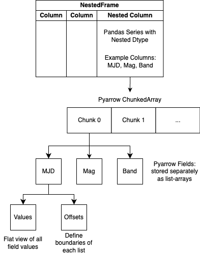
Internals: Powering Efficient Data Analysis with `pyarrow`#

“Dataframes within Dataframes” is a useful hueristic for understanding the API/workings of a NestedFrame. However, the actual storage representation leverages pyarrow (a package that contains a set of technologies that enable data systems to efficiently store, process, and move data) and materializes the nested dataframes as a view of the data. The following diagram details the actual storage representation of nested-pandas:

5cfbef1b7df84fd088077b057ea52de2

Performance Impact of `nested-pandas`#

The design of nested-pandas yields significant speedups over using pandas native workflows in many cases. Below is a brief example workflow comparison between pandas and nested-pandas, where this example workflow calculates the amplitude of fluxes after a few filtering steps.

`pandas`#

[8]:

%%timeit

# Read data
object_df = pd.read_parquet("objects.parquet")
source_df = pd.read_parquet("ztf_sources.parquet")

# Filter on object
filtered_object = object_df.query("ra > 10.0")
#sync object to source --removes any index values of source not found in object
filtered_source = filtered_object[[]].join(source_df, how="left")

# Count number of observations per photometric band and add it to the object table
band_counts = source_df.groupby(level=0).apply(lambda x:
                                               x[["band"]].value_counts().reset_index()).pivot_table(values="count",
                                                                                                     index="index",
                                                                                                     columns="band",
                                                                                                     aggfunc="sum")
filtered_object = filtered_object.join(band_counts[["g","r"]])

# Filter on our nobs
filtered_object = filtered_object.query("g > 520")
filtered_source = filtered_object[[]].join(source_df, how="left")

# Calculate Amplitude
amplitude = licu.Amplitude()
filtered_source.groupby(level=0).apply(lambda x: amplitude(np.array(x.mjd), np.array(x.flux)))

492 ms ± 3.87 ms per loop (mean ± std. dev. of 7 runs, 1 loop each)

`nested-pandas`#

[9]:

%%timeit

#Read in parquet data
#nesting sources into objects
nf = npd.read_parquet(data="objects.parquet",
                  to_pack={"ztf_sources": "ztf_sources.parquet"})

# Filter on object
nf = nf.query("ra > 10.0")

# Count number of observations per photometric band and add it as a column
nf = npd.utils.count_nested(nf, "ztf_sources", by="band", join=True)

# Filter on our nobs
nf = nf.query("n_ztf_sources_g > 520")

# Calculate Amplitude
amplitude = licu.Amplitude()
nf.reduce(amplitude, "ztf_sources.mjd", "ztf_sources.flux")

227 ms ± 4.74 ms per loop (mean ± std. dev. of 7 runs, 1 loop each)

In this example, nested-pandas has improved the speed of computation by ~2x and also reduced the overall code footprint of the workflow. As a relatively simple workflow, this is a conservative example of the performance gains of nested-pandas as in more complex workflows we expect to see more and more joins and groupbys in a native pandas workflow that are avoided in nested-pandas.

Addressing Scale: `nested-dask`#

The row-by-row optimizations introduced in nested-pandas are vital to efficiently work at scale. However, just as pandas is largely limited to in-memory datasets, so is nested-pandas.

dask is a package that equips pandas with the ability to work at scale, by:

Providing built-in parallelization and larger-than-memory computation of workflows
Introducing “lazy” computation, where operations are tracked and run only when data is needed/requested
Providing dashboarding utility to help users monitor/debug their active workflows

This motivates the LINCC-Frameworks package, nested-dask, to bring the efficiency gains of nested-pandas to the scale of Rubin.

`nested-dask` Showcase: Eclipsing Binary Search in the PLAsTiCC Dataset#

The API of nested-dask follows the API of Nested-Pandas closely, and as such we’ll show nested-dask

The goal of the workflow is to identify a subset of eclipsing binary candidates within the dataset.

Photometric LSST Astronomical Time-Series Classification Challenge (PLAsTiCC)

3,492,890 Objects
453,653,104 Sources

[10]:

# Setting up a Dask Client allows us to define the used compute resources
from dask.distributed import Client
client = Client(n_workers=4,
                dashboard_address=':39876')

# Not available externally
DATA_DIR = "/Users/dbranton/lincc/timeseries/data/plasticc/parquet"

client

[10]:

Client

Client-93b5aef0-e978-11ef-a6bc-62679ec975a9

Connection method: Cluster object	Cluster type: distributed.LocalCluster
Dashboard: http://127.0.0.1:39876/status

Cluster Info

LocalCluster

0501abeb

Dashboard: http://127.0.0.1:39876/status	Workers: 4
Total threads: 12	Total memory: 32.00 GiB
Status: running	Using processes: True

Scheduler Info

Scheduler

Scheduler-d76311e4-6ab5-481f-ab82-18d5c5ced2cd

Comm: tcp://127.0.0.1:51402	Workers: 4
Dashboard: http://127.0.0.1:39876/status	Total threads: 12
Started: Just now	Total memory: 32.00 GiB

Workers

Worker: 0

Comm: tcp://127.0.0.1:51413	Total threads: 3
Dashboard: http://127.0.0.1:51414/status	Memory: 8.00 GiB
Nanny: tcp://127.0.0.1:51405
Local directory: /var/folders/lc/dws63_cs5gz5mf8s869hjpx40000gn/T/dask-scratch-space/worker-z1j2dur9

Worker: 1

Comm: tcp://127.0.0.1:51416	Total threads: 3
Dashboard: http://127.0.0.1:51417/status	Memory: 8.00 GiB
Nanny: tcp://127.0.0.1:51407
Local directory: /var/folders/lc/dws63_cs5gz5mf8s869hjpx40000gn/T/dask-scratch-space/worker-siq69g1f

Worker: 2

Comm: tcp://127.0.0.1:51419	Total threads: 3
Dashboard: http://127.0.0.1:51420/status	Memory: 8.00 GiB
Nanny: tcp://127.0.0.1:51409
Local directory: /var/folders/lc/dws63_cs5gz5mf8s869hjpx40000gn/T/dask-scratch-space/worker-qvayg4hg

Worker: 3

Comm: tcp://127.0.0.1:51422	Total threads: 3
Dashboard: http://127.0.0.1:51423/status	Memory: 8.00 GiB
Nanny: tcp://127.0.0.1:51411
Local directory: /var/folders/lc/dws63_cs5gz5mf8s869hjpx40000gn/T/dask-scratch-space/worker-k8apqymq

[11]:

%%time
# Load in Plasticc data
object_ndf = nd.read_parquet(DATA_DIR+"/object/*.parquet",
                         dtype_backend="pyarrow",
                         index="object_id",
                         calculate_divisions=True,
                         columns=["ra", "decl","hostgal_photoz"])
source_ndf = nd.read_parquet(DATA_DIR+"/source/*.parquet",
                         dtype_backend="pyarrow",
                         index="object_id",
                         calculate_divisions=True,)

# Nesting Sources in Object
objsor_ndf = object_ndf.add_nested(source_ndf, "source")

CPU times: user 43.7 ms, sys: 15.9 ms, total: 59.6 ms
Wall time: 65.1 ms

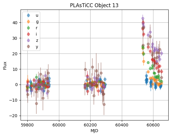
[12]:

# Grab the source dataframe for the first object
obj = objsor_ndf.head(1).iloc[0]
lc = obj.source

for band in np.unique(lc.passband):
    band_mask = lc.passband == band
    band_labels = ["u","g","r","i","z","y"]
    plt.errorbar(lc.mjd[band_mask],
                 lc.flux[band_mask],
                 yerr=lc.flux_err[band_mask],
                 fmt='o', alpha=0.5,
                 label=band_labels[band])

plt.title(f"PLAsTiCC Object {obj.name}")
plt.ylabel("Flux")
plt.xlabel("MJD")
plt.grid()
plt.legend()

[12]:

<matplotlib.legend.Legend at 0x176a93b00>

../../_images/notebooks_nested_review_demo_30_1.png

First, let’s select only Galactic objects, by cutting on redshift:

[13]:

%%time
objsor_ndf = objsor_ndf.query("hostgal_photoz < 0.001")

CPU times: user 12.5 ms, sys: 2.97 ms, total: 15.5 ms
Wall time: 18.6 ms

Second, let’s select persistent sources, by cutting on the duration of the light curve:

[14]:

%%time
def calc_ptp(time, detected):
    try:
        return {"duration": np.ptp(time[np.asarray(detected, dtype=bool)])}
    except ValueError:
        return {"duration": 0}

duration = objsor_ndf.reduce(calc_ptp, 'source.mjd', 'source.detected_bool',
                         meta={"duration":"float"})
# Filter by the calculated duration
objsor_ndf = objsor_ndf.assign(duration=duration["duration"])
objsor_ndf = objsor_ndf.query("duration > 366")

CPU times: user 22.1 ms, sys: 3.59 ms, total: 25.7 ms
Wall time: 27.2 ms

Next, we use Otsu’s method to split light curves into two groups: one with high flux, and one with low flux. Eclipsing binaries should have lower flux group smaller than the higher flux group, but having larger variability. For simplicity, we only calculate these features for the i (3) band.

[15]:

%%time

def otsu_fmt(*args, **kwargs):
    otsu = licu.OtsuSplit()
    res = otsu(*args, **kwargs)
    return {'otsu_mean_diff': res[0],
           'otsu_std_lower': res[1],
           'otsu_std_upper': res[2],
            'otsu_lower_to_all_ratio': res[3]}

objsor_ndf_3 = objsor_ndf.query("source.passband == 3")
otsu_features = objsor_ndf_3.reduce(otsu_fmt, 'source.mjd', 'source.flux',
                               meta={'otsu_mean_diff': float,
                                     'otsu_std_lower': float,
                                     'otsu_std_upper': float,
                                     'otsu_lower_to_all_ratio': float,})
# Assign Columns
objsor_ndf = objsor_ndf.assign(
    otsu_lower_to_all_ratio=otsu_features['otsu_lower_to_all_ratio'],
    otsu_std_lower=otsu_features['otsu_std_lower'],
    otsu_std_upper=otsu_features['otsu_std_upper'],
)
# Filter by Otsu Features
objsor_ndf = objsor_ndf.query(
    "otsu_lower_to_all_ratio < 0.1 and otsu_std_lower > otsu_std_upper",
)

CPU times: user 25.3 ms, sys: 3.57 ms, total: 28.9 ms
Wall time: 27.5 ms

And finally, we can call compute to kick off the computation:

[16]:

%%time
objsor_df = objsor_ndf.compute()

CPU times: user 2.62 s, sys: 649 ms, total: 3.27 s
Wall time: 9.44 s

Note: Our previous LINCC-Frameworks project, Timeseries Analysis & Processing Engine (TAPE), completed this workflow in ~45 seconds using the same cluster setup. TAPE serves as a rough expectation of native pandas performance, as it utilized the pandas/dask dataframe API for its operations

[17]:

objsor_df.sort_values(by="duration")

[17]:

decl

hostgal_photoz

source

duration

otsu_lower_to_all_ratio

otsu_std_lower

otsu_std_upper

object_id

5018697

89.278100

-55.299400

0.000000

mjd	passband	flux	flux_err	detected_bool

59581.0517

19.395758

19.307962

145 rows × 5 columns

366.026900

0.090909

20.334780

11.308998

107162588

103.183600

-27.279600

0.000000

59583.344

9.877261

21.849825

146 rows × 5 columns

366.945900

0.083333

59.450195

13.847480

81231667

79.804700

-36.609200

0.000000

59583.1166

-14.752371

12.623836

138 rows × 5 columns

367.078500

0.086957

18.588678

12.536847

70340192

33.966300

-51.255800

0.000000

59796.3661

3.669538

3.129773

137 rows × 5 columns

367.819400

0.086957

15.041311

7.034880

19873025

318.164100

-19.629600

0.000000

59728.3383

-8.527591

11.58319

128 rows × 5 columns

368.225900

0.090909

61.010877

5.875888

...

4354 rows x 8 columns

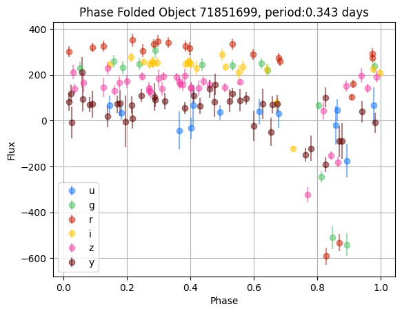
[18]:

# Grab the source dataframe for the first object
obj = objsor_df.loc[71851699] #71851699
lc = obj.source

model = LombScargleMultiband(lc.mjd, lc.flux, lc.passband, lc.flux_err, nterms_base=2, nterms_band=1)
frequency, power = model.autopower(method='flexible', nyquist_factor=50)
freq_maxpower = frequency[np.argmax(power)]
t_phase = np.linspace(0, 1/freq_maxpower, 100)
y_fit = model.model(t_phase, freq_maxpower)

COLORS = {'u': '#0c71ff', 'g': '#49be61', 'r': '#c61c00',
          'i': '#ffc200', 'z': '#f341a2', 'y': '#5d0000'}

#plt.plot(frequency, power)

for band in np.unique(lc.passband):
    band_mask = lc.passband == band
    band_labels = ["u","g","r","i","z","y"]
    #plt.plot(t_phase/(1/freq_maxpower), y_fit[band], '-', color=COLORS[band_labels[band]])
    plt.errorbar(lc.mjd[band_mask]%(1/freq_maxpower)/(1/freq_maxpower),
                 lc.flux[band_mask],
                 yerr=lc.flux_err[band_mask],
                 fmt='o', alpha=0.5,
                 label=band_labels[band],
                 color=COLORS[band_labels[band]])

plt.title(f"Phase Folded Object {obj.name}, period:{np.round(1/freq_maxpower,3)} days")
plt.ylabel("Flux")
plt.xlabel("Phase")
plt.grid()
plt.legend()

[18]:

<matplotlib.legend.Legend at 0x35071f740>

../../_images/notebooks_nested_review_demo_41_1.png

[ ]:

nested-pandas/nested-dask Demonstration

Contents

`nested-pandas`/`nested-dask` Demonstration#

`nested-pandas` Overview#

The NestedFrame Interface#

Applying Operations Directly to Nested Data#

Run Custom User Functions with `reduce`#

Internals: Powering Efficient Data Analysis with `pyarrow`#

Performance Impact of `nested-pandas`#

`pandas`#

`nested-pandas`#

Addressing Scale: `nested-dask`#

`nested-dask` Showcase: Eclipsing Binary Search in the PLAsTiCC Dataset#

Client

Cluster Info

LocalCluster

Scheduler Info

Scheduler

Workers

Worker: 0

Worker: 1

Worker: 2

Worker: 3

nested-pandas/nested-dask Demonstration

Contents

nested-pandas/nested-dask Demonstration#

nested-pandas Overview#

The NestedFrame Interface#

Applying Operations Directly to Nested Data#

Run Custom User Functions with reduce#

Internals: Powering Efficient Data Analysis with pyarrow#

Performance Impact of nested-pandas#

pandas#

nested-pandas#

Addressing Scale: nested-dask#

nested-dask Showcase: Eclipsing Binary Search in the PLAsTiCC Dataset#

Client

Cluster Info

LocalCluster

Scheduler Info

Scheduler

Workers

Worker: 0

Worker: 1

Worker: 2

Worker: 3

`nested-pandas`/`nested-dask` Demonstration#

`nested-pandas` Overview#

Run Custom User Functions with `reduce`#

Internals: Powering Efficient Data Analysis with `pyarrow`#

Performance Impact of `nested-pandas`#

`pandas`#

`nested-pandas`#

Addressing Scale: `nested-dask`#

`nested-dask` Showcase: Eclipsing Binary Search in the PLAsTiCC Dataset#